Accelerating simulations through deep pondering on symbolic propagation
Last month I attended a summer school for one week at the super compute center (PDC) at KTH. One hot topic in scientific computing today is how to utilize the new low precision hardware that is being rolled out now. Actually it seems that high precision hardware is being rolled in, which is troublesome since scientific computing relies on it. One topic that has been bothering me for quite some time is why scientific computing has failed to deliver long range the predictions of both micro- and macroscopic systems that are being solved by “oracle methods” today, such as the protein folding and weather forecasting problems. I had an interesting discussion about this with several researchers at the school. As it turns out, the main reason why classical simulations has failed to solve it is simply because of the immense amount of computational resources required to do it. Simple as that.
Why does it require such immense computing power? Microscopic systems are described by quantum mechanics, and ideally these should be solved from first principles by ab initio molecular dynamics simulations, which is at it’s highest level, divided into two steps. First, one computes energies by performing a so called single point simulation, using either quantum chemistry (i.e. solve the Schrödinger equation under the Born-Oppenheimer approximation) or density functional theory, to iteratively obtain the (ground state) energy of the system using self consistent field equations. Usually one has to apply various approximations here already, such as ignoring the inner shell electrons (giving rise to a so called pseudopotential). If that is too exact one can resort to using a force field approximation where the many body exchange and correlation interactions are replaced with an empirical two-body interaction. Once the energy is obtained, then one updates the atom positions by calculating the forces from the energy gradient (which is allowed due to the Hellman-Feynman theorem). Atoms in a protein in water at room temperature oscillate at a frequency in the femtohertz range, usually around 10-100 THz ($\sim 10^{13}$-$10^{14}$ Hz). These two steps must be performed at a sampling frequency at least twice (some authors recommend starting with four times 1) that of the oscillation frequency, otherwise information is lost à la Nyquist sampling theorem (though it is a bit more complex than this). Since the simulation must be performed at this minuscule time scale, we simply do not have the resources today to simulate such a system long enough. Since the tractable sampling time is so short, simulating so called rare events is highly unlikely to happen. These rare events might be crucial to understand why a system acts the way it does at longer time scales, and missing to simulate these puts a fundamental limitation on what can be predicted in the long run. The success of black box artificial intelligence to solve the long term behavior without going through the rare events should be of the greatest curiosity in computational chemistry, but it should also trigger thoughts on how we can match these predictions using white box ab initio simulations such that we can gain scientific knowledge from it.
One key take away from the course is that compute is getting increasingly cheap, but memory operations are still lagging behind. Hence, if you can reformulate a memory access in terms of a recompute, that is cheap on modern hardware. This made me think, can we accelerate simulations by reformulating the dynamics somehow, to utilize the compute resources better?
Contents
- Simulations
- Shallow water equations
- Symbolic expression propagation
- Deep pondering
- Rounding up
- Appendix
Simulations
What is a simulation? You define some sort of state $s$ and differential equation that relates time to space through a (most likely non-linear) operator $F$, call it the propagator
$$ \frac{\partial s}{\partial t} = F[s] $$
The propagator is a higher order function; it’s application is denoted with square brackets. In integral form the term “propagator” becomes more clear, as it defines how a state evolves over time
$$ s(t,x) = \int_0^t F[s](t,x) dt $$
This is fundamentally what a simulation try to solve. Note that the integral is a linear operator and can be decomposed by subdivision of the interval of integration. Let’s drop the nuisance parameter $x$ for notational convenience
$$ s(t_{i+1}) = \Bigg(\int_0^{t_i} + \int_{t_i}^{t_{i+1}}\Bigg) F[s](t) dt = s(t_i) + \int_{t_i}^{t_{i+1}} F[s](t) dt $$
So the state $s(t_{i+1})$ at a time in the future can be determined from the state $s(t_i)$ now. This decomposition property allows us to solve the integral in discrete steps. If the step is taken small enough such that $t_{i+1} = t_i + dt$ we can approximate $F[s](t) \, \forall t \in [t,t+dt]$ as locally constant such that
$$ \int_{t_i}^{t_{i+1}} F[s](t)dt = \int_{t_i}^{t_i+dt} F[s](t) dt \approx F[s](t_i) dt $$
which yields the Euler integration scheme
$$ s(t_{i+1}) = s(t_i) + F[s](t_i)dt $$
which is just one out of many ways to approximate the fundamental integral equation. It should be said that this procedure is not good for production code for several reasons. First of all, it is not stable at larger time scales, and is not be used for serious numerical work. Secondly, it does not conserve certain physical invariants, such as time reversal symmetry; if you take one step forward and then one step back (with derivatives evaluated from the source location), you will not end up in the same place! Nevertheless it will be the method of choice in this post; partially due to it’s simplicity, partially due to my non-expertise in numerics.
Now the system is discretized in time, but it is still continuous in space. Let us define a sampling operator, or in short, a sampler $S$ which maps continuous functions to discrete, and acts on integrals by converting them to finite sums and maps continuous derivatives to finite differences on some pre-specified grid $\{ x_k | k \in \mathbb{Z} \}$. The most simple sampler is the dirac sampler, defined as
$$ S[s](k) = \int s(x) \delta(x - x_k)dx = s(x_k) $$
It is worth emphasizing that this sampler is not possible to realize for any physical sensor, but can sometimes be a good approximation. In the sensor fusion literature one talks about measurement models. For a more physically plausible sampler you would at least have to incorporate noise (usually gaussian) and integrate over time (sample and hold). For an image sensor noise is better described with poisson statistics, and integration is to be performed over both pixel area and exposure time. In this post, we define it to act on integrals as defined above in the Euler integration scheme, and on the first order derivative as follows
$$\begin{align} S \Bigg[ \int_a^b F[s](t,x) dt \Bigg] &= s(a,x) + (b-a)S\{F\}[s](a,x) \newline S \bigg\{ \frac{\partial}{\partial x} \bigg\} s(t,x) &= S\bigg[\frac{\partial s}{\partial x}\bigg](t,x) = \frac{s(t,x+dx) - s(t,x-dx)}{2dx} \end{align}$$
I have introduced a notation with braces $\{\cdot\}$ to distinguish application to operators from application to functions (as denoted with brackets $[\cdot]$). Thus the expression “sampling the propagator and applying to the state” $S\{F\}[s]$ and sampling the propagated state $S\big[F[s]\big]$ are both valid and mean the same thing. Note that this is just one out of many ways to sample differential and integral expressions; using different samplers give rise to different numerical methods. The selection of points $(x-dx, x+dx)$ around the center $x$ is known as the stencil. Simulating the system can then be done by discretizing over both time and space and numerically propagate these equations. Let $s_i(k) = s(t_i, x_k)$, then we can define the first order difference operator $D$ as
$$ D[s_i](k) \equiv S\bigg[\frac{\partial s}{\partial x}\bigg](t_i,x_k) = \frac{s_i(k+1) - s_i(k-1)}{2dx} $$
The system is then simulated by applying the sampling operator to the Euler integration scheme
$$ s_{i+1} = s_{i} + S\{F\}[s_i]dt $$
When the type of the operand of the propagator can be inferred from context one can relax the notation a bit, and drop the explicit application of the sampler to the continuous state, and just work with the discrete state directly. Applying an operator to a discrete state should then be interpreted with a sampler implicitly applied. Introducing the updator (a.k.a update operator) one can just write
$$ s_{i+1} = U[s_i] = s_{i} + F[s_i]dt $$
where $F$ is now the discretized propagator acting on the discrete state $s_i = s(t_i, x_k)$. I hope this notational excursion does not occlude my intents here. I want to illustrate that approximating a continuous system with a discrete one is a non-trivial task, and I want to be clear about the problem this post is attacking and under what assumptions. The goal is to explore ways to accelerate the recursive application of the updator in different ways. As a first attempt, let’s focus on combining two steps into one and derive $U^2 = U \circ U$.
Shallow water equations
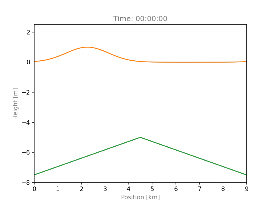
As a toy problem, let us analyze a simplified version of the shallow water equations (a.k.a. Saint-Venant equations 2) in one dimension. Why these? Because they are simple and fun to watch! The equations are
$$\begin{align} \frac{dh}{dt} &= - \frac{d}{dx}\big((A + h)v\big) = - \bigg[ (A + h)\frac{dv}{dx} + v\bigg(\frac{dA}{dx} + \frac{dh}{dx}\bigg) \bigg] \newline \frac{dv}{dt} &= - \bigg[ G\frac{dh}{dx} + v\frac{dv}{dx} \bigg] \end{align}$$
where $A$ is the water depth, $h$ is the surface height displacement and $v$ is the horizontal water velocity. Simulating the system can be done by discretizing over time with a step duration $dt$ on a grid with step length $dx$, and numerically integrating these equations as described in the previous section. Defining discrete propagators $F_h$ and $F_v$ for each variable in the state $s = (h,v)$, then the Euler step becomes
$$\begin{align} h_{i+1} &= U_h[h_i,v_i] = h_i + F_h[h_i,v_i]dt = h_i - dt \Big( (A + h_i) D[v_i] + v_i \big( D[A] + D[h_i] \big) \Big) \newline v_{i+1} &= U_v[h_i,v_i] = v_i + F_v[h_i,v_i]dt = v_i - dt \Big( G D[h_i] + v_i D[v_i] \Big) \end{align}$$
The joint system updator is defined as the operator performing
$$ U[h_i, v_i] \rightarrow (h_{i+1}, v_{i+1}) = (U_h[h_i, v_i], U_v[h_i, v_i]) $$
Simulating the system would then look something as follows in Fortran. Let the arrays be allocated with custom bounds between $-1$ and $n+1$ to accommodate so called “halo points”. The boundary conditions are set to be circular to keep things simple.
do t = 1, steps
    ! Populate halo points
    h(-1)  = h(n)
    h(n+1) = h(0)
    ! Compute gradients
    dh_dx(0:n) = diff(h,dx)
    dv_dx(0:n) = diff(v,dx)
    ! Compute tendencies
    dh_dt = -(A + h)*dv_dx - v*(dA_dx + dh_dx)
    dv_dt = -G*dh_dx - v*dv_dx
    ! Update
    h = h + dt*dh_dt
    v = v + dt*dv_dt
end do
Where the finite differences looks something like this
function diff(f,dx) result(df_dx)
    real, intent(in) :: f(:), dx
    real :: df_dx(size(f)-2), eta
    integer :: n
    n = size(f)
    eta = 0.5 / dx
    df_dx = eta*(f(3:n) - f(1:n-2))
end function diff
The recursive computational graph looks as follows, where the constants $G$ and $A$ have been excluded for brevity, since they do not affect the dependencies formed between computational steps
Unrolling it for two time steps it looks like
That looks complex, but it should be obvious that the variables $h$ and $v$ in iteration 3 can be expressed solely in terms of various orders of derivatives of the variables in iteration 1. This is exactly the property that we are looking for, replacing memory dependencies with more computations! To avoid ambiguity, let $\tilde U$ denote the updator of the continuous state. There are essentially two ways we can obtain a updator from $h_1$ and $v_1$ to $h_3$ and $v_3$ directly without going through $h_2$ and $v_2$
- Compose the one step discrete updator with itself: $S(\tilde U)^2 = S(\tilde U) \circ S(\tilde U)$.
- Discretize the composition of a one step continuous updator with itself: $S(\tilde U^2) = S(\tilde U \circ \tilde U)$
The first approach is guaranteed (up to floating point errors) to give the same results as performing the original simulation. The second will actually yield new discrete dynamics as we will see later.
Applying the updator and looking at the state at position $k$ and dropping time subscripts and use an assignment notation instead we obtain the recursive rewrite rule
$$\begin{align} h(k) &\leftarrow h(k) - dt \bigg( \big( A(k) + h(k) \big)\frac{v(k+1) - v(k-1)}{2 dx} + v(k) \frac{A(k+1)-A(k-1)+h(k+1)-h(k-1)}{2dx} \bigg) \newline &= h(k) - \frac{dt}{2 dx} \bigg( \big( A(k) + h(k) \big)\big(v(k+1) - v(k-1)\big) + v(k) \big( A(k+1)-A(k-1)+h(k+1)-h(k-1) \big) \bigg) \newline &= h(k) - \eta \bigg( A(k)v(k+1) - A(k)v(k-1) + h(k)v(k+1) - h(k)v(k-1) + v(k)A(k+1) - v(k)A(k-1) + v(k)h(k+1) - v(k)h(k-1) \bigg) \newline v(k) &\leftarrow v(k) - dt \bigg( G\frac{h(k+1) - h(k-1)}{2 dx} + v(k)\frac{v(k+1) - v(k-1)}{2 dx} \bigg) \newline &= v(k) - \eta \bigg( G\big(h(k+1) - h(k-1)\big) + v(k)\big(v(k+1) - v(k-1)\big) \bigg) \newline \end{align}$$
where the intrinsic step size $\eta = dt/2dx$ has been introduced. The update can be described by the following computational graph
By performing the rewrite twice we obtain $U^2$. The rewrite is easy to do with a computer algebra system such as SymPy. However, it should be noted that there is a risk of exponential term explosion here since $h(x)$ rewrites to 8 terms and $v(x)$ to 4, so the joint state $s(x) = \big(h(x), v(x)\big)$ rewrites to 12 terms, and one could expect the double substitution to produce up to 144 terms! The generated equations are not suitable for human consumption but is better processed by the computer. Problem is that expressions can be simplified in so many ways, and computer algebra systems need guidance from us to identify symmetries. One such symmetry is the natural step factored out from the propagator sub-expression earlier.
Symbolic expression propagation
In order to evaluate the performance of different updator expressions, we need a generic interface to code against. I wrote a generic simulation environment module in Fortran for doing this, with an updator interface that one can plug in various solutions. The module code is given in the appendix. Now, to test an updator one just has to write a minimal program that “use” the simulator module, initialize it by specifying the required padding (that is, the number of neighboring elements one need in a local update step), and supply a function satisfying the updator interface. The baseline code shown earlier rewritten on updator forms becomes
program main
  use simulator
  implicit none

  real(flt), allocatable :: dA(:), dh(:), dv(:)

  call init(1)
  call alloc(dA,1)
  call alloc(dh,1)
  call alloc(dv,1)
  dA(0:n) = diff(A)
  call prepare(A)
  call simulate(1, update)

contains
  subroutine update(h1, v1, h2, v2)
    real(flt), contiguous, intent(in)  :: h1(-1:), v1(-1:)
    real(flt), contiguous, intent(out) :: h2(-1:), v2(-1:)
    dh = diff(h1)
    dv = diff(v1)
    h2 = h1 - eta*((A + h1)*dv + v1*(dA + dh))
    v2 = v1 - eta*(G*dh + v1*dv)
  end subroutine update

  pure function diff(f) result(df)
    real(flt), contiguous, intent(in) :: f(-1:)
    real(flt) :: df(-1:n+1)
    df(0:n) = f(1:n+1) - f(-1:n-1)
  end function diff
end program main
Manually rolling out the loop performed by the vector expression into a sequence of scalar expressions the code simplifies somewhat
program main
  use simulator
  implicit none

  call init(1)
  call simulate(1, update)

contains
  subroutine update(h, v, h2, v2)
    real(flt), contiguous, intent(in)  :: h(-1:) , v(-1:)
    real(flt), contiguous, intent(out) :: h2(-1:), v2(-1:)
    integer :: k
    do concurrent (k = 0:n)
      h2(k) = (eta*(A(k)*v(k - 1) + A(k - 1)*v(k) + h(k)*v(k - 1) + h(k - 1)*v(k) - A(k)*v(k + 1) - A(k + 1)*v(k) - h(k)*v(k + 1) - h(k + 1)*v(k)) + h(k))
      v2(k) = (eta*(G*h(k - 1) + v(k)*v(k - 1) - G*h(k + 1) - v(k)*v(k + 1)) + v(k))
    end do
  end subroutine
end program main
Running the code and visualizing it with the provided script in the appendix the results looks like this

Pretty cool huh? It simulates for 30 minutes because the shallow water equations can not describe breaking waves, which happens after 30 min, which manifest itself by creating unphysical ripples
that you can see start forming at the end of the simulation.
Somewhat surprisingly, the scalar version is faster than the vector version on my computer.
I compiled the code with aggressive optimization flags (-Ofast) to let the compiler optimize things freely.
Since I have not built the expressions with numerical stability in mind I can let the compiler do whatever it thinks can improve the performance.
The vector version takes about 1.6 seconds to execute, while the scalar version only 1.1 seconds. That is almost a 50% speedup already!
I haven’t studied the generated assembly code, but I guess the compiler fails to inline certain subexpressions and write things back and forth to memory,
and perhaps fails to fuse the vector operations into one loop.
Due to this observation I will not use vector expressions in subsequent code, but always use the unrolled scalar version.
Two step updator
Alright, with the simulator environment setup, let us analyse the first option outlined earlier and compose the one step discrete updator. The updator expression is computed by the computer algebra system by propagating symbols, or in short, symprop. This gives a large $\eta^3$ order expression which is not shown here but directly pasted into a Fortran program (I don’t expect you to read the code, it’s just provided for reference)
program main
  use simulator
  implicit none

  call init(2)
  call simulate(2, update)

contains
  subroutine update(h, v, h2, v2)
    real(flt), contiguous, intent(in)  :: h(-2:), v(-2:)
    real(flt), contiguous, intent(out) :: h2(-2:), v2(-2:)
    integer :: k
    do concurrent (k = 0:n)
      h2(k) = (eta*((eta*(G*h(k - 1) + v(k)*v(k - 1) - G*h(k + 1) - v(k)*v(k + 1)) + v(k))*(eta*(A(k - 1)*v(k - 2) + A(k - 2)*v(k - 1) + h(k - 1)*v(k - 2) + h(k - 2)*v(k - 1) - A(k)*v(k - 1) - A(k - 1)*v(k) - h(k)*v(k - 1) - h(k - 1)*v(k)) + h(k - 1)) + (eta*(G*h(k - 1) + v(k)*v(k - 1) - G*h(k + 1) - v(k)*v(k + 1)) + v(k))*A(k - 1) + (eta*(G*h(k - 2) + v(k - 1)*v(k - 2) - G*h(k) - v(k)*v(k - 1)) + v(k - 1))*(eta*(A(k)*v(k - 1) + A(k - 1)*v(k) + h(k)*v(k - 1) + h(k - 1)*v(k) - A(k)*v(k + 1) - A(k + 1)*v(k) - h(k)*v(k + 1) - h(k + 1)*v(k)) + h(k)) + (eta*(G*h(k - 2) + v(k - 1)*v(k - 2) - G*h(k) - v(k)*v(k - 1)) + v(k - 1))*A(k) - (eta*(G*h(k) + v(k)*v(k + 1) - G*h(k + 2) - v(k + 1)*v(k + 2)) + v(k + 1))*(eta*(A(k)*v(k - 1) + A(k - 1)*v(k) + h(k)*v(k - 1) + h(k - 1)*v(k) - A(k)*v(k + 1) - A(k + 1)*v(k) - h(k)*v(k + 1) - h(k + 1)*v(k)) + h(k)) - (eta*(G*h(k) + v(k)*v(k + 1) - G*h(k + 2) - v(k + 1)*v(k + 2)) + v(k + 1))*A(k) - (eta*(G*h(k - 1) + v(k)*v(k - 1) - G*h(k + 1) - v(k)*v(k + 1)) + v(k))*(eta*(A(k)*v(k + 1) + A(k + 1)*v(k) + h(k)*v(k + 1) + h(k + 1)*v(k) - A(k + 1)*v(k + 2) - A(k + 2)*v(k + 1) - h(k + 1)*v(k + 2) - h(k + 2)*v(k + 1)) + h(k + 1)) - (eta*(G*h(k - 1) + v(k)*v(k - 1) - G*h(k + 1) - v(k)*v(k + 1)) + v(k))*A(k + 1)) + eta*(A(k)*v(k - 1) + A(k - 1)*v(k) + h(k)*v(k - 1) + h(k - 1)*v(k) - A(k)*v(k + 1) - A(k + 1)*v(k) - h(k)*v(k + 1) - h(k + 1)*v(k)) + h(k))
      v2(k) = (eta*(G*(eta*(A(k - 1)*v(k - 2) + A(k - 2)*v(k - 1) + h(k - 1)*v(k - 2) + h(k - 2)*v(k - 1) - A(k)*v(k - 1) - A(k - 1)*v(k) - h(k)*v(k - 1) - h(k - 1)*v(k)) + h(k - 1)) + (eta*(G*h(k - 1) + v(k)*v(k - 1) - G*h(k + 1) - v(k)*v(k + 1)) + v(k))*(eta*(G*h(k - 2) + v(k - 1)*v(k - 2) - G*h(k) - v(k)*v(k - 1)) + v(k - 1)) - G*(eta*(A(k)*v(k + 1) + A(k + 1)*v(k) + h(k)*v(k + 1) + h(k + 1)*v(k) - A(k + 1)*v(k + 2) - A(k + 2)*v(k + 1) - h(k + 1)*v(k + 2) - h(k + 2)*v(k + 1)) + h(k + 1)) - (eta*(G*h(k) + v(k)*v(k + 1) - G*h(k + 2) - v(k + 1)*v(k + 2)) + v(k + 1))*(eta*(G*h(k - 1) + v(k)*v(k - 1) - G*h(k + 1) - v(k)*v(k + 1)) + v(k))) + eta*(G*h(k - 1) + v(k)*v(k - 1) - G*h(k + 1) - v(k)*v(k + 1)) + v(k))
    end do
  end subroutine
end program main
Now let us analyse the second option; sampling the two step continuous propagator. The updates in continuous space form are
$$\begin{align} h_2 &= h_1 - dt \bigg( (A + h_1)\frac{dv_1}{dx} + v_1 \Big( \frac{dh_1}{dx} + \frac{dA}{dx} \Big) \bigg) \newline v_2 &= v_1 - dt \bigg( G\frac{dh_1}{dx} + v_1\frac{dv_1}{dx} \bigg) \newline h_3 &= h_2 - dt \bigg( (A + h_2)\frac{dv_2}{dx} + v_2 \Big( \frac{dh_2}{dx} + \frac{dA}{dx} \Big) \bigg) \newline v_3 &= v_2 - dt \bigg( G\frac{dh_2}{dx} + v_2\frac{dv_2}{dx} \bigg) \newline \end{align}$$
The derivatives are computed as
$$\begin{align} \frac{dh_2}{dx} &= \frac{d}{dx} \Bigg( h_1 - dt \bigg( (A + h_1)\frac{dv_1}{dx} + v_1 \Big( \frac{dA}{dx} + \frac{dh_1}{dx} \Big) \bigg) \Bigg) \newline &= \frac{dh_1}{dx} - dt \bigg( (A + h_1)\frac{d^2v_1}{dx^2} + 2 \Big(\frac{dA}{dx} + \frac{dh_1}{dx} \Big) \frac{dv_1}{dx} + v_1 \Big(\frac{d^2A}{dx^2} + \frac{d^2h_1}{dx^2} \Big) \bigg) \newline \frac{dv_2}{dx} &= \frac{d}{dx} \Bigg( v_1 - dt \bigg( G\frac{dh_1}{dx} + v_1\frac{dv_1}{dx} \bigg) \Bigg) = \frac{dv_1}{dx} - dt \bigg( G\frac{d^2h_1}{dx^2} + v_1\frac{d^2v_1}{dx^2} + \Big(\frac{dv_1}{dx}\Big)^2 \bigg) \end{align}$$
Let us define the sampling of the second order differential, the second order difference operator, as
$$ D^2[s](k) \equiv S\bigg[\frac{\partial^2 s}{\partial x^2}\bigg](x_k) = \frac{s(k+1) - 2s(k) + s(k-1)}{2dx^2} $$
which is used to rewrite all occurrences of continuous derivatives to discrete form. This gives a large $\eta^3$ order expression just like the first order two step updator shown earlier, which we also paste directly into the Fortran program below
program main
use simulator
implicit none

call init(2)
call simulate(2, update)

contains
  subroutine update(h, v, h2, v2)
    real(flt), contiguous, intent(in)  :: h(-2:), v(-2:)
    real(flt), contiguous, intent(out) :: h2(-2:), v2(-2:)
    integer :: k
    do concurrent (k = 0:n)
      h2(k) = (eta*((-v(k + 1) + v(k - 1))*(A(k) + h(k)) + (-A(k + 1) - h(k + 1) + A(k - 1) + h(k - 1))*v(k)) + eta*((eta*(G*(-h(k + 1) + h(k - 1)) + (-v(k + 1) + v(k - 1))*v(k)) + v(k))*(-A(k + 1) - h(k + 1) + 2*eta*(-(-v(k + 1) + v(k - 1))*(-A(k - 1) - h(k - 1) + A(k + 1) + h(k + 1)) + 2*(A(k) + h(k))*(-2*v(k) + v(k + 1) + v(k - 1)) + 2*(-2*A(k) - 2*h(k) + A(k + 1) + A(k - 1) + h(k + 1) + h(k - 1))*v(k)) + A(k - 1) + h(k - 1)) + (-v(k + 1) + eta*((-v(k + 1) + v(k - 1))**2 + 4*G*(-2*h(k) + h(k + 1) + h(k - 1)) + 4*(-2*v(k) + v(k + 1) + v(k - 1))*v(k)) + v(k - 1))*(eta*((-v(k + 1) + v(k - 1))*(A(k) + h(k)) + (-A(k + 1) - h(k + 1) + A(k - 1) + h(k - 1))*v(k)) + A(k) + h(k))) + h(k))
      v2(k) = (eta*(G*(-h(k + 1) + h(k - 1)) + (-v(k + 1) + v(k - 1))*v(k)) + eta*(G*(-h(k + 1) + 2*eta*(-(-v(k + 1) + v(k - 1))*(-A(k - 1) - h(k - 1) + A(k + 1) + h(k + 1)) + 2*(A(k) + h(k))*(-2*v(k) + v(k + 1) + v(k - 1)) + 2*(-2*A(k) - 2*h(k) + A(k + 1) + A(k - 1) + h(k + 1) + h(k - 1))*v(k)) + h(k - 1)) + (eta*(G*(-h(k + 1) + h(k - 1)) + (-v(k + 1) + v(k - 1))*v(k)) + v(k))*(-v(k + 1) + eta*((-v(k + 1) + v(k - 1))**2 + 4*G*(-2*h(k) + h(k + 1) + h(k - 1)) + 4*(-2*v(k) + v(k + 1) + v(k - 1))*v(k)) + v(k - 1))) + v(k))
    end do
  end subroutine
end program main
The first order version runs in about 1.2s, so slightly slower than the baseline, but the second order method runs in about 0.8s, which is faster! The reason for this is probably because the first order updator has a receptive field of $\pm 2$ units around the center, while the second order method just needs the $\pm 1$ nearest neighbors, accessing less memory and doing more compute, which is what we want to do. The simulation results are shown below for reference


Three step updator
Motivated by the results from the two step continuous updator, let us try the three step updator obtained by sampling the third order derivative as follows
$$ S\bigg[\frac{\partial^3 s}{\partial{x^3}}\bigg](x) = \frac{s(x+2dx) - 2s(x+dx) + 2s(x-dx) - s(x-2dx)}{2dx^3} $$
The generated update expression is huge has terms up to $\eta^7$. The program is given below for reference.
program main
use simulator
implicit none

call init(3)
call simulate(3, update)

contains

subroutine update(h, v, h2, v2)
    real(flt), contiguous, intent(in)  :: h(-3:), v(-3:)
    real(flt), contiguous, intent(out) :: h2(-3:), v2(-3:)
    integer :: k
    do concurrent (k = 0:n)
        h2(k) = (eta*((-v(k + 1) + v(k - 1))*(A(k) + h(k)) + (-A(k + 1) - h(k + 1) + A(k - 1) + h(k - 1))*v(k)) + eta*((eta*(G*(-h(k + 1) + h(k - 1)) + (-v(k + 1) + v(k - 1))*v(k)) + v(k))*(-A(k + 1) - h(k + 1) + 2*eta*(-(-v(k + 1) + v(k - 1))*(-A(k - 1) - h(k - 1) + A(k + 1) + h(k + 1)) + 2*(A(k) + h(k))*(-2*v(k) + v(k + 1) + v(k - 1)) + 2*(-2*A(k) - 2*h(k) + A(k + 1) + A(k - 1) + h(k + 1) + h(k - 1))*v(k)) + A(k - 1) + h(k - 1)) + (-v(k + 1) + eta*((-v(k + 1) + v(k - 1))**2 + 4*G*(-2*h(k) + h(k + 1) + h(k - 1)) + 4*(-2*v(k) + v(k + 1) + v(k - 1))*v(k)) + v(k - 1))*(eta*((-v(k + 1) + v(k - 1))*(A(k) + h(k)) + (-A(k + 1) - h(k + 1) + A(k - 1) + h(k - 1))*v(k)) + A(k) + h(k))) + eta*((eta*(G*(-h(k + 1) + h(k - 1)) + (-v(k + 1) + v(k - 1))*v(k)) + eta*(G*(-h(k + 1) + 2*eta*((-v(k - 1) + v(k + 1))*(-A(k - 1) - h(k - 1) + A(k + 1) + h(k + 1)) + 2*(A(k) + h(k))*(-2*v(k) + v(k + 1) + v(k - 1)) + 2*(-2*A(k) - 2*h(k) + A(k + 1) + A(k - 1) + h(k + 1) + h(k - 1))*v(k)) + h(k - 1)) - (-v(k) + eta*(G*(-h(k - 1) + h(k + 1)) + (-v(k - 1) + v(k + 1))*v(k)))*(-v(k + 1) + eta*((-v(k - 1) + v(k + 1))**2 + 4*G*(-2*h(k) + h(k + 1) + h(k - 1)) + 4*(-2*v(k) + v(k + 1) + v(k - 1))*v(k)) + v(k - 1))) + v(k))*(-A(k + 1) - h(k + 1) - eta*((-v(k) + eta*(G*(-h(k - 1) + h(k + 1)) + (-v(k - 1) + v(k + 1))*v(k)))*(-8*A(k) - 8*h(k) + 4*A(k + 1) + 4*A(k - 1) + 4*h(k + 1) + 4*h(k - 1) - eta*((-A(k - 3) - h(k - 3) - 3*A(k + 1) - 3*h(k + 1) + 3*A(k - 1) + 3*h(k - 1) + A(k + 3) + h(k + 3))*v(k) - (A(k) + h(k))*(-v(k + 3) - 3*v(k - 1) + 3*v(k + 1) + v(k - 3)) - 12*(-v(k + 1) + v(k - 1))*(-2*A(k) - 2*h(k) + A(k + 1) + A(k - 1) + h(k + 1) + h(k - 1)) + 12*(-2*v(k) + v(k + 1) + v(k - 1))*(-A(k - 1) - h(k - 1) + A(k + 1) + h(k + 1)))) + (-eta*((-A(k - 1) - h(k - 1) + A(k + 1) + h(k + 1))*v(k) - (-v(k + 1) + v(k - 1))*(A(k) + h(k))) + A(k) + h(k))*(-4*v(k + 1) - 4*v(k - 1) + 8*v(k) + eta*(G*(-h(k - 3) - 3*h(k + 1) + 3*h(k - 1) + h(k + 3)) + (-v(k - 3) - 3*v(k + 1) + 3*v(k - 1) + v(k + 3))*v(k) + 12*(-v(k - 1) + v(k + 1))*(-2*v(k) + v(k + 1) + v(k - 1)))) + 2*(-v(k + 1) + eta*((-v(k - 1) + v(k + 1))**2 + 4*G*(-2*h(k) + h(k + 1) + h(k - 1)) + 4*(-2*v(k) + v(k + 1) + v(k - 1))*v(k)) + v(k - 1))*(-A(k - 1) - h(k - 1) - 2*eta*(-(-v(k + 1) + v(k - 1))*(-A(k - 1) - h(k - 1) + A(k + 1) + h(k + 1)) + 2*(A(k) + h(k))*(-2*v(k) + v(k + 1) + v(k - 1)) + 2*(-2*A(k) - 2*h(k) + A(k + 1) + A(k - 1) + h(k + 1) + h(k - 1))*v(k)) + A(k + 1) + h(k + 1))) + 2*eta*((-v(k + 1) + v(k - 1))*(-A(k + 1) - h(k + 1) + A(k - 1) + h(k - 1)) + 2*(A(k) + h(k))*(-2*v(k) + v(k + 1) + v(k - 1)) + 2*(-2*A(k) - 2*h(k) + A(k + 1) + A(k - 1) + h(k + 1) + h(k - 1))*v(k)) + A(k - 1) + h(k - 1)) + (-v(k + 1) + eta*((-v(k + 1) + v(k - 1))**2 + 4*G*(-2*h(k) + h(k + 1) + h(k - 1)) + 4*(-2*v(k) + v(k + 1) + v(k - 1))*v(k)) + eta*((-v(k + 1) + eta*((-v(k + 1) + v(k - 1))**2 + 4*G*(-2*h(k) + h(k + 1) + h(k - 1)) + 4*(-2*v(k) + v(k + 1) + v(k - 1))*v(k)) + v(k - 1))**2 - G*(-4*h(k + 1) - 4*h(k - 1) + 8*h(k) + eta*((-A(k - 3) - h(k - 3) - 3*A(k + 1) - 3*h(k + 1) + 3*A(k - 1) + 3*h(k - 1) + A(k + 3) + h(k + 3))*v(k) - (A(k) + h(k))*(-v(k + 3) - 3*v(k - 1) + 3*v(k + 1) + v(k - 3)) - 12*(-v(k + 1) + v(k - 1))*(-2*A(k) - 2*h(k) + A(k + 1) + A(k - 1) + h(k + 1) + h(k - 1)) + 12*(-2*v(k) + v(k + 1) + v(k - 1))*(-A(k - 1) - h(k - 1) + A(k + 1) + h(k + 1)))) - (eta*(G*(-h(k + 1) + h(k - 1)) + (-v(k + 1) + v(k - 1))*v(k)) + v(k))*(-4*v(k + 1) - 4*v(k - 1) + 8*v(k) - eta*(G*(-h(k + 3) - 3*h(k - 1) + 3*h(k + 1) + h(k - 3)) + (-v(k + 3) - 3*v(k - 1) + 3*v(k + 1) + v(k - 3))*v(k) + 12*(-v(k + 1) + v(k - 1))*(-2*v(k) + v(k + 1) + v(k - 1))))) + v(k - 1))*(eta*((-v(k) + eta*(G*(-h(k - 1) + h(k + 1)) + (-v(k - 1) + v(k + 1))*v(k)))*(-A(k - 1) - h(k - 1) - 2*eta*(-(-v(k + 1) + v(k - 1))*(-A(k - 1) - h(k - 1) + A(k + 1) + h(k + 1)) + 2*(A(k) + h(k))*(-2*v(k) + v(k + 1) + v(k - 1)) + 2*(-2*A(k) - 2*h(k) + A(k + 1) + A(k - 1) + h(k + 1) + h(k - 1))*v(k)) + A(k + 1) + h(k + 1)) + (-v(k + 1) + eta*((-v(k - 1) + v(k + 1))**2 + 4*G*(-2*h(k) + h(k + 1) + h(k - 1)) + 4*(-2*v(k) + v(k + 1) + v(k - 1))*v(k)) + v(k - 1))*(-eta*((-A(k - 1) - h(k - 1) + A(k + 1) + h(k + 1))*v(k) - (-v(k + 1) + v(k - 1))*(A(k) + h(k))) + A(k) + h(k))) + eta*((-v(k + 1) + v(k - 1))*(A(k) + h(k)) + (-A(k + 1) - h(k + 1) + A(k - 1) + h(k - 1))*v(k)) + A(k) + h(k))) + h(k))
        v2(k) = (eta*(G*(-h(k + 1) + h(k - 1)) + (-v(k + 1) + v(k - 1))*v(k)) + eta*(G*(-h(k + 1) + 2*eta*(-(-v(k + 1) + v(k - 1))*(-A(k - 1) - h(k - 1) + A(k + 1) + h(k + 1)) + 2*(A(k) + h(k))*(-2*v(k) + v(k + 1) + v(k - 1)) + 2*(-2*A(k) - 2*h(k) + A(k + 1) + A(k - 1) + h(k + 1) + h(k - 1))*v(k)) + h(k - 1)) + (eta*(G*(-h(k + 1) + h(k - 1)) + (-v(k + 1) + v(k - 1))*v(k)) + v(k))*(-v(k + 1) + eta*((-v(k + 1) + v(k - 1))**2 + 4*G*(-2*h(k) + h(k + 1) + h(k - 1)) + 4*(-2*v(k) + v(k + 1) + v(k - 1))*v(k)) + v(k - 1))) + eta*(G*(-h(k + 1) - eta*((-v(k) + eta*(G*(-h(k - 1) + h(k + 1)) + (-v(k - 1) + v(k + 1))*v(k)))*(-8*A(k) - 8*h(k) + 4*A(k + 1) + 4*A(k - 1) + 4*h(k + 1) + 4*h(k - 1) - eta*((-A(k - 3) - h(k - 3) - 3*A(k + 1) - 3*h(k + 1) + 3*A(k - 1) + 3*h(k - 1) + A(k + 3) + h(k + 3))*v(k) - (A(k) + h(k))*(-v(k + 3) - 3*v(k - 1) + 3*v(k + 1) + v(k - 3)) - 12*(-v(k + 1) + v(k - 1))*(-2*A(k) - 2*h(k) + A(k + 1) + A(k - 1) + h(k + 1) + h(k - 1)) + 12*(-2*v(k) + v(k + 1) + v(k - 1))*(-A(k - 1) - h(k - 1) + A(k + 1) + h(k + 1)))) + (-eta*((-A(k - 1) - h(k - 1) + A(k + 1) + h(k + 1))*v(k) - (-v(k + 1) + v(k - 1))*(A(k) + h(k))) + A(k) + h(k))*(-4*v(k + 1) - 4*v(k - 1) + 8*v(k) + eta*(G*(-h(k - 3) - 3*h(k + 1) + 3*h(k - 1) + h(k + 3)) + (-v(k - 3) - 3*v(k + 1) + 3*v(k - 1) + v(k + 3))*v(k) + 12*(-v(k - 1) + v(k + 1))*(-2*v(k) + v(k + 1) + v(k - 1)))) + 2*(-v(k + 1) + eta*((-v(k - 1) + v(k + 1))**2 + 4*G*(-2*h(k) + h(k + 1) + h(k - 1)) + 4*(-2*v(k) + v(k + 1) + v(k - 1))*v(k)) + v(k - 1))*(-A(k - 1) - h(k - 1) - 2*eta*(-(-v(k + 1) + v(k - 1))*(-A(k - 1) - h(k - 1) + A(k + 1) + h(k + 1)) + 2*(A(k) + h(k))*(-2*v(k) + v(k + 1) + v(k - 1)) + 2*(-2*A(k) - 2*h(k) + A(k + 1) + A(k - 1) + h(k + 1) + h(k - 1))*v(k)) + A(k + 1) + h(k + 1))) + 2*eta*(-(-v(k + 1) + v(k - 1))*(-A(k - 1) - h(k - 1) + A(k + 1) + h(k + 1)) + 2*(A(k) + h(k))*(-2*v(k) + v(k + 1) + v(k - 1)) + 2*(-2*A(k) - 2*h(k) + A(k + 1) + A(k - 1) + h(k + 1) + h(k - 1))*v(k)) + h(k - 1)) - (-v(k) + eta*((-v(k) + eta*(G*(-h(k - 1) + h(k + 1)) + (-v(k - 1) + v(k + 1))*v(k)))*(-v(k + 1) + eta*((-v(k - 1) + v(k + 1))**2 + 4*G*(-2*h(k) + h(k + 1) + h(k - 1)) + 4*(-2*v(k) + v(k + 1) + v(k - 1))*v(k)) + v(k - 1)) - G*(-h(k + 1) + 2*eta*((-v(k - 1) + v(k + 1))*(-A(k - 1) - h(k - 1) + A(k + 1) + h(k + 1)) + 2*(A(k) + h(k))*(-2*v(k) + v(k + 1) + v(k - 1)) + 2*(-2*A(k) - 2*h(k) + A(k + 1) + A(k - 1) + h(k + 1) + h(k - 1))*v(k)) + h(k - 1))) - eta*(G*(-h(k + 1) + h(k - 1)) + (-v(k + 1) + v(k - 1))*v(k)))*(-v(k + 1) + eta*((-v(k + 1) + v(k - 1))**2 + 4*G*(-2*h(k) + h(k + 1) + h(k - 1)) + 4*(-2*v(k) + v(k + 1) + v(k - 1))*v(k)) + eta*((-v(k + 1) + eta*((-v(k - 1) + v(k + 1))**2 + 4*G*(-2*h(k) + h(k + 1) + h(k - 1)) + 4*(-2*v(k) + v(k + 1) + v(k - 1))*v(k)) + v(k - 1))**2 + (-v(k) + eta*(G*(-h(k - 1) + h(k + 1)) + (-v(k - 1) + v(k + 1))*v(k)))*(-4*v(k + 1) - 4*v(k - 1) + 8*v(k) + eta*(G*(-h(k - 3) - 3*h(k + 1) + 3*h(k - 1) + h(k + 3)) + (-v(k - 3) - 3*v(k + 1) + 3*v(k - 1) + v(k + 3))*v(k) + 12*(-v(k - 1) + v(k + 1))*(-2*v(k) + v(k + 1) + v(k - 1)))) - G*(-4*h(k + 1) - 4*h(k - 1) + 8*h(k) + eta*((A(k) + h(k))*(-v(k - 3) - 3*v(k + 1) + 3*v(k - 1) + v(k + 3)) + (-A(k - 3) - h(k - 3) - 3*A(k + 1) - 3*h(k + 1) + 3*A(k - 1) + 3*h(k - 1) + A(k + 3) + h(k + 3))*v(k) + 12*(-v(k - 1) + v(k + 1))*(-2*A(k) - 2*h(k) + A(k + 1) + A(k - 1) + h(k + 1) + h(k - 1)) + 12*(-2*v(k) + v(k + 1) + v(k - 1))*(-A(k - 1) - h(k - 1) + A(k + 1) + h(k + 1))))) + v(k - 1))) + v(k))
    end do
end subroutine

end program main
Unfortunately, it does not improve performance but runs around 1.7s on my computer, slightly slower than the baseline. I believe this is partly due to the sheer number of new terms in the unrolled expression; partly due to the receptive field expanding from $\pm 1$ to $\pm 2$ elements just like the first order two step updator. I tried to optimize the expression manually in several ways, but failed miserably. While trying to optimize it I quickly learned that it’s beneficial to preserve as much as possible of the computational structure when handing it over to the compiler. Giving the compiler an expanded expression performs awfully bad (about half a magnitude slower), probably because the compiler (gfortran in my case), while allowed to perform any kind of “unsafe math optimization” such as redistributing or reassociating expressions, it will not refactor them. Factoring expressions can be very time consuming, and a compiler is not allowed to spend arbitrary time pondering on such things. It might perform better if implemented on an accelerator, but it might also perform even worse, it really depends on how well the compiler can optimize it and perform register allocation for each subexpression. The combinatorial explosion in number of terms is a big limitation to this approach, which I will tackle in the next section.
Going beyond three steps
Composing the updator $N$ times will give rise to terms on the form $\eta^r$ for $r \in \{0,1,…,2^N-1\}$. Question is, do we need all those terms? If we simulate with small enough time step $dt$ or large enough space step $dx$ such that $\eta \ll 0$, then we might be able to approximate $\eta^r \approx 0$ for large enough $r$. However, reducing the temporal step size $dt$ counteracts what we are trying to do in the first place; to reduce the number of steps! Naturally, expanding to “$r$:th order” will include all elements up to $\log_2(r)$ steps back in time, and start throwing away elements for steps beyond that (though in a non-trivial fashion). So let us see how the expansion of the second order updator to second order looks like
$$\begin{align} h(k) \leftarrow h{\left(k \right)} &+ \eta \left(2 A{\left(k \right)} v{\left(k - 1 \right)} - 2 A{\left(k \right)} v{\left(k + 1 \right)} + 2 A{\left(k - 1 \right)} v{\left(k \right)} - 2 A{\left(k + 1 \right)} v{\left(k \right)} + 2 h{\left(k \right)} v{\left(k - 1 \right)} - 2 h{\left(k \right)} v{\left(k + 1 \right)} + 2 h{\left(k - 1 \right)} v{\left(k \right)} - 2 h{\left(k + 1 \right)} v{\left(k \right)}\right) \newline &+ \eta^{2} \left(- 2 G A{\left(k \right)} h{\left(k \right)} + G A{\left(k \right)} h{\left(k - 2 \right)} + G A{\left(k \right)} h{\left(k + 2 \right)} + G A{\left(k - 1 \right)} h{\left(k - 1 \right)} - G A{\left(k - 1 \right)} h{\left(k + 1 \right)} - G A{\left(k + 1 \right)} h{\left(k - 1 \right)} + G A{\left(k + 1 \right)} h{\left(k + 1 \right)} - 2 G h^{2}{\left(k \right)} + G h{\left(k \right)} h{\left(k - 2 \right)} + G h{\left(k \right)} h{\left(k + 2 \right)} + G h^{2}{\left(k - 1 \right)} - 2 G h{\left(k - 1 \right)} h{\left(k + 1 \right)} + G h^{2}{\left(k + 1 \right)} - 2 A{\left(k \right)} v{\left(k \right)} v{\left(k - 1 \right)} - 2 A{\left(k \right)} v{\left(k \right)} v{\left(k + 1 \right)} + A{\left(k \right)} v{\left(k - 2 \right)} v{\left(k - 1 \right)} + A{\left(k \right)} v^{2}{\left(k - 1 \right)} - 2 A{\left(k \right)} v{\left(k - 1 \right)} v{\left(k + 1 \right)} + A{\left(k \right)} v^{2}{\left(k + 1 \right)} + A{\left(k \right)} v{\left(k + 1 \right)} v{\left(k + 2 \right)} + A{\left(k - 2 \right)} v{\left(k \right)} v{\left(k - 1 \right)} - A{\left(k - 1 \right)} v^{2}{\left(k \right)} + A{\left(k - 1 \right)} v{\left(k \right)} v{\left(k - 2 \right)} + 2 A{\left(k - 1 \right)} v{\left(k \right)} v{\left(k - 1 \right)} - 2 A{\left(k - 1 \right)} v{\left(k \right)} v{\left(k + 1 \right)} - A{\left(k + 1 \right)} v^{2}{\left(k \right)} - 2 A{\left(k + 1 \right)} v{\left(k \right)} v{\left(k - 1 \right)} + 2 A{\left(k + 1 \right)} v{\left(k \right)} v{\left(k + 1 \right)} + A{\left(k + 1 \right)} v{\left(k \right)} v{\left(k + 2 \right)} + A{\left(k + 2 \right)} v{\left(k \right)} v{\left(k + 1 \right)} - 2 h{\left(k \right)} v{\left(k \right)} v{\left(k - 1 \right)} - 2 h{\left(k \right)} v{\left(k \right)} v{\left(k + 1 \right)} + h{\left(k \right)} v{\left(k - 2 \right)} v{\left(k - 1 \right)} + h{\left(k \right)} v^{2}{\left(k - 1 \right)} - 2 h{\left(k \right)} v{\left(k - 1 \right)} v{\left(k + 1 \right)} + h{\left(k \right)} v^{2}{\left(k + 1 \right)} + h{\left(k \right)} v{\left(k + 1 \right)} v{\left(k + 2 \right)} + h{\left(k - 2 \right)} v{\left(k \right)} v{\left(k - 1 \right)} - h{\left(k - 1 \right)} v^{2}{\left(k \right)} + h{\left(k - 1 \right)} v{\left(k \right)} v{\left(k - 2 \right)} + 2 h{\left(k - 1 \right)} v{\left(k \right)} v{\left(k - 1 \right)} - 2 h{\left(k - 1 \right)} v{\left(k \right)} v{\left(k + 1 \right)} - h{\left(k + 1 \right)} v^{2}{\left(k \right)} - 2 h{\left(k + 1 \right)} v{\left(k \right)} v{\left(k - 1 \right)} + 2 h{\left(k + 1 \right)} v{\left(k \right)} v{\left(k + 1 \right)} + h{\left(k + 1 \right)} v{\left(k \right)} v{\left(k + 2 \right)} + h{\left(k + 2 \right)} v{\left(k \right)} v{\left(k + 1 \right)}\right) + O\left(\eta^{3}\right) \newline &+ \mathcal{O(\eta^3)} \newline v(k) \leftarrow v{\left(k \right)} &+ \eta \left(2 G h{\left(k - 1 \right)} - 2 G h{\left(k + 1 \right)} + 2 v{\left(k \right)} v{\left(k - 1 \right)} - 2 v{\left(k \right)} v{\left(k + 1 \right)}\right) \newline &+ \eta^{2} \left(- G A{\left(k \right)} v{\left(k - 1 \right)} - G A{\left(k \right)} v{\left(k + 1 \right)} + G A{\left(k - 2 \right)} v{\left(k - 1 \right)} - G A{\left(k - 1 \right)} v{\left(k \right)} + G A{\left(k - 1 \right)} v{\left(k - 2 \right)} - G A{\left(k + 1 \right)} v{\left(k \right)} + G A{\left(k + 1 \right)} v{\left(k + 2 \right)} + G A{\left(k + 2 \right)} v{\left(k + 1 \right)} - 2 G h{\left(k \right)} v{\left(k \right)} - G h{\left(k \right)} v{\left(k - 1 \right)} - G h{\left(k \right)} v{\left(k + 1 \right)} + G h{\left(k - 2 \right)} v{\left(k \right)} + G h{\left(k - 2 \right)} v{\left(k - 1 \right)} - G h{\left(k - 1 \right)} v{\left(k \right)} + G h{\left(k - 1 \right)} v{\left(k - 2 \right)} + G h{\left(k - 1 \right)} v{\left(k - 1 \right)} - G h{\left(k - 1 \right)} v{\left(k + 1 \right)} - G h{\left(k + 1 \right)} v{\left(k \right)} - G h{\left(k + 1 \right)} v{\left(k - 1 \right)} + G h{\left(k + 1 \right)} v{\left(k + 1 \right)} + G h{\left(k + 1 \right)} v{\left(k + 2 \right)} + G h{\left(k + 2 \right)} v{\left(k \right)} + G h{\left(k + 2 \right)} v{\left(k + 1 \right)} - v^{2}{\left(k \right)} v{\left(k - 1 \right)} - v^{2}{\left(k \right)} v{\left(k + 1 \right)} + v{\left(k \right)} v{\left(k - 2 \right)} v{\left(k - 1 \right)} + v{\left(k \right)} v^{2}{\left(k - 1 \right)} - 2 v{\left(k \right)} v{\left(k - 1 \right)} v{\left(k + 1 \right)} + v{\left(k \right)} v^{2}{\left(k + 1 \right)} + v{\left(k \right)} v{\left(k + 1 \right)} v{\left(k + 2 \right)}\right) + O\left(\eta^{3}\right) \newline &+ \mathcal{O(\eta^3)} \newline \end{align}$$
There about twice as many third order terms as second order, so this really is monster of an expression! Instead of bluntly truncating it, we can estimate an upper bound on each term and truncate only if we are satisfying certain conditions. One trivial upper bound is to rewrite all terms
$$\begin{align} h(\cdot) &\leftarrow h = \max (h(k-1), h(k), h(k+1)) \newline v(\cdot) &\leftarrow v = \max(v(k-1), v(k), v(k+1)) \end{align}$$
which gives an upper bound on the magnitude of the assignments
$$\begin{align} h &\leftarrow \eta^{3} \cdot \left(32 A G h v + 24 A v^{3} + 30 G h^{2} v + 24 h v^{3}\right) + \eta^{2} \cdot \left(8 A G h + 24 A v^{2} + 8 G h^{2} + 24 h v^{2}\right) + \eta \left(8 A v + 8 h v\right) + h \newline v &\leftarrow \eta^{3} \cdot \left(8 G^{2} h^{2} + 16 G h v^{2} + 6 v^{4}\right) + \eta^{2} \cdot \left(8 A G v + 16 G h v + 8 v^{3}\right) + \eta \left(4 G h + 4 v^{2}\right) + v \end{align}$$
A term $c_r \eta^r$ can be truncated if $c_r \eta^r \ll 1$. How much smaller than unity it must be depends on required accuracy $\varepsilon$. This gives us a truncation condition on the form
$$ c_r \leq \frac{\varepsilon}{\eta^r} $$
With the bounds check in mind, let us for the moment assume that $c_r \eta^r \leq \varepsilon \, \forall r \ge 2$ and truncate all higher order terms beyond second order. Applying this approximation to the third order updator from last section gives the truncated third order three step updator
$$\begin{align} h(k) \leftarrow h(k) &+ \eta \left(3 A{\left(k \right)} v{\left(k - 1 \right)} - 3 A{\left(k \right)} v{\left(k + 1 \right)} + 3 A{\left(k - 1 \right)} v{\left(k \right)} - 3 A{\left(k + 1 \right)} v{\left(k \right)} + 3 h{\left(k \right)} v{\left(k - 1 \right)} - 3 h{\left(k \right)} v{\left(k + 1 \right)} + 3 h{\left(k - 1 \right)} v{\left(k \right)} - 3 h{\left(k + 1 \right)} v{\left(k \right)}\right) \newline &+ \eta^{2} \left(- 24 G A{\left(k \right)} h{\left(k \right)} + 12 G A{\left(k \right)} h{\left(k - 1 \right)} + 12 G A{\left(k \right)} h{\left(k + 1 \right)} + 3 G A{\left(k - 1 \right)} h{\left(k - 1 \right)} - 3 G A{\left(k - 1 \right)} h{\left(k + 1 \right)} - 3 G A{\left(k + 1 \right)} h{\left(k - 1 \right)} + 3 G A{\left(k + 1 \right)} h{\left(k + 1 \right)} - 24 G h^{2}{\left(k \right)} + 12 G h{\left(k \right)} h{\left(k - 1 \right)} + 12 G h{\left(k \right)} h{\left(k + 1 \right)} + 3 G h^{2}{\left(k - 1 \right)} - 6 G h{\left(k - 1 \right)} h{\left(k + 1 \right)} + 3 G h^{2}{\left(k + 1 \right)} - 72 A{\left(k \right)} v^{2}{\left(k \right)} + 24 A{\left(k \right)} v{\left(k \right)} v{\left(k - 1 \right)} + 24 A{\left(k \right)} v{\left(k \right)} v{\left(k + 1 \right)} + 6 A{\left(k \right)} v^{2}{\left(k - 1 \right)} - 12 A{\left(k \right)} v{\left(k - 1 \right)} v{\left(k + 1 \right)} + 6 A{\left(k \right)} v^{2}{\left(k + 1 \right)} + 12 A{\left(k - 1 \right)} v^{2}{\left(k \right)} + 12 A{\left(k - 1 \right)} v{\left(k \right)} v{\left(k - 1 \right)} - 12 A{\left(k - 1 \right)} v{\left(k \right)} v{\left(k + 1 \right)} + 12 A{\left(k + 1 \right)} v^{2}{\left(k \right)} - 12 A{\left(k + 1 \right)} v{\left(k \right)} v{\left(k - 1 \right)} + 12 A{\left(k + 1 \right)} v{\left(k \right)} v{\left(k + 1 \right)} - 72 h{\left(k \right)} v^{2}{\left(k \right)} + 24 h{\left(k \right)} v{\left(k \right)} v{\left(k - 1 \right)} + 24 h{\left(k \right)} v{\left(k \right)} v{\left(k + 1 \right)} + 6 h{\left(k \right)} v^{2}{\left(k - 1 \right)} - 12 h{\left(k \right)} v{\left(k - 1 \right)} v{\left(k + 1 \right)} + 6 h{\left(k \right)} v^{2}{\left(k + 1 \right)} + 12 h{\left(k - 1 \right)} v^{2}{\left(k \right)} + 12 h{\left(k - 1 \right)} v{\left(k \right)} v{\left(k - 1 \right)} - 12 h{\left(k - 1 \right)} v{\left(k \right)} v{\left(k + 1 \right)} + 12 h{\left(k + 1 \right)} v^{2}{\left(k \right)} - 12 h{\left(k + 1 \right)} v{\left(k \right)} v{\left(k - 1 \right)} + 12 h{\left(k + 1 \right)} v{\left(k \right)} v{\left(k + 1 \right)}\right) \newline v(k) \leftarrow v(k) &+ \eta \left(3 G h{\left(k - 1 \right)} - 3 G h{\left(k + 1 \right)} + 3 v{\left(k \right)} v{\left(k - 1 \right)} - 3 v{\left(k \right)} v{\left(k + 1 \right)}\right) \newline &+ \eta^{2} \left(- 48 G A{\left(k \right)} v{\left(k \right)} + 12 G A{\left(k \right)} v{\left(k - 1 \right)} + 12 G A{\left(k \right)} v{\left(k + 1 \right)} + 12 G A{\left(k - 1 \right)} v{\left(k \right)} + 6 G A{\left(k - 1 \right)} v{\left(k - 1 \right)} - 6 G A{\left(k - 1 \right)} v{\left(k + 1 \right)} + 12 G A{\left(k + 1 \right)} v{\left(k \right)} - 6 G A{\left(k + 1 \right)} v{\left(k - 1 \right)} + 6 G A{\left(k + 1 \right)} v{\left(k + 1 \right)} - 72 G h{\left(k \right)} v{\left(k \right)} + 12 G h{\left(k \right)} v{\left(k - 1 \right)} + 12 G h{\left(k \right)} v{\left(k + 1 \right)} + 24 G h{\left(k - 1 \right)} v{\left(k \right)} + 9 G h{\left(k - 1 \right)} v{\left(k - 1 \right)} - 9 G h{\left(k - 1 \right)} v{\left(k + 1 \right)} + 24 G h{\left(k + 1 \right)} v{\left(k \right)} - 9 G h{\left(k + 1 \right)} v{\left(k - 1 \right)} + 9 G h{\left(k + 1 \right)} v{\left(k + 1 \right)} - 24 v^{3}{\left(k \right)} + 12 v^{2}{\left(k \right)} v{\left(k - 1 \right)} + 12 v^{2}{\left(k \right)} v{\left(k + 1 \right)} + 6 v{\left(k \right)} v^{2}{\left(k - 1 \right)} - 12 v{\left(k \right)} v{\left(k - 1 \right)} v{\left(k + 1 \right)} + 6 v{\left(k \right)} v^{2}{\left(k + 1 \right)}\right) \end{align}$$
Note that we have dropped all terms with $\eta^r$ for $r > 2$ all the way up to 7. How does this perform? Let us compare with the exact third order updator (from last section).


There is no observable difference! Unfortunately, the truncated version executes slower (2.2s) than the exact third order updator (1.7s) due to expression expansion when truncating higher order terms. Fully expanding the expression as a series in $\eta$ and then truncating it leads to even worse performance (as learned when implementing the exact third order updator earlier), so I had to implement a graph preserving truncation algorithm, where as much as possible of the original computation graph is kept while throwing away higher order terms. It might be possible to improve this, as my implementation completely expand multiplications, which could be done partially in some way to lose less structure.
However, note that the receptive field has decreased from $\pm 2$ to $\pm 1$ when truncating higher order terms. In general, truncating to r:th order removes any terms beyond the (spatial) r-nearest neighbors, maintaining the receptive field to $\pm r$. Truncating to second order means we need to maintain the stencil $(-2,-1,0,+1,+2)$. This motivates us to try composing truncated updators, since they will always have a small receptive field but have an increasingly longer “lookahead” in time. From now on, I will be implicit with the truncation level (which is 2) and the continuous derivative order (which is three) and only talk in terms of how many steps an updator performs in one go. Also, since we are approximating things now, let us to a slight shift in terminology and refer to the updators as predictors instead. Let us start with the four step predictor (which is to be interpreted as the truncated third order four step predictor). It runs in 2s, slightly faster than the third step predictor. What about 8-step? It runs in 1s! 16-step? You guessed it, 0.5s. Ok, but does it predict the correct results? Have a look yourself! Below is a comparison between the exact three step updator and the 16-step predictor

There is still no observable difference in the simulated time interval! It is at this point that I got really excited. But hold on, how does this compare to simply multiplying the step size by 16 in the one step updator, and then skip every 16 steps, making a naive first order 16-step predictor? Turns out that it still works fine for this specific simulation, but things go bad when you multiply with 32. So how does the 32 step predictor compare to the “naive 32 step predictor” obtained by multiplying $\eta$ by 32? It is still stable!


How far ahead into the future can we predict? I composed the predictors up to 256 steps before it collapses at 512. It took around 15 minutes of “pondering” to derive it (I’ll come back to this term later).

With the 256-step predictor the simulation runs more than 30x faster than the baseline, and 2x faster than the than what could be achieved by naively increasing the time step size. The code for all predictors are given in the appendix. How does the expressions look like? The coefficients are interesting, there is a trivial sequence for the first order terms but there is no obvious pattern for the second order terms except for an approximate 4x growth in each step. Let us look at the coefficients for the $v$ state for a different lookaheads
$$\begin{align} \hat v_{4} (k) &= v{\left(k \right)} &&+ \eta \left(- 4 v{\left(k \right)} v{\left(k+1 \right)} + 4 v{\left(k \right)} v{\left(k-1 \right)} - 4 G h{\left(k+1 \right)} + 4 G h{\left(k-1 \right)}\right) &&+ \eta^{2} \left(3 v{\left(k \right)} v{\left(k+1 \right)} v{\left(k+2 \right)} + 9 v{\left(k \right)} v^{2}{\left(k+1 \right)} - 18 v{\left(k \right)} v{\left(k-1 \right)} v{\left(k+1 \right)} + 9 v{\left(k \right)} v^{2}{\left(k-1 \right)} + 3 v{\left(k \right)} v{\left(k-2 \right)} v{\left(k-1 \right)} + 9 v^{2}{\left(k \right)} v{\left(k+1 \right)} + 9 v^{2}{\left(k \right)} v{\left(k-1 \right)} - 24 v^{3}{\left(k \right)} + 3 G h{\left(k+2 \right)} v{\left(k+1 \right)} + 3 G h{\left(k+2 \right)} v{\left(k \right)} + 3 G h{\left(k+1 \right)} v{\left(k+2 \right)} + 12 G h{\left(k+1 \right)} v{\left(k+1 \right)} - 12 G h{\left(k+1 \right)} v{\left(k-1 \right)} + 21 G h{\left(k+1 \right)} v{\left(k \right)} - 12 G h{\left(k-1 \right)} v{\left(k+1 \right)} + 12 G h{\left(k-1 \right)} v{\left(k-1 \right)} + 3 G h{\left(k-1 \right)} v{\left(k-2 \right)} + 21 G h{\left(k-1 \right)} v{\left(k \right)} + 3 G h{\left(k-2 \right)} v{\left(k-1 \right)} + 3 G h{\left(k-2 \right)} v{\left(k \right)} + 9 G h{\left(k \right)} v{\left(k+1 \right)} + 9 G h{\left(k \right)} v{\left(k-1 \right)} - 78 G h{\left(k \right)} v{\left(k \right)} + 3 G A{\left(k+2 \right)} v{\left(k+1 \right)} + 3 G A{\left(k+1 \right)} v{\left(k+2 \right)} + 6 G A{\left(k+1 \right)} v{\left(k+1 \right)} - 6 G A{\left(k+1 \right)} v{\left(k-1 \right)} + 9 G A{\left(k+1 \right)} v{\left(k \right)} - 6 G A{\left(k-1 \right)} v{\left(k+1 \right)} + 6 G A{\left(k-1 \right)} v{\left(k-1 \right)} + 3 G A{\left(k-1 \right)} v{\left(k-2 \right)} + 9 G A{\left(k-1 \right)} v{\left(k \right)} + 3 G A{\left(k-2 \right)} v{\left(k-1 \right)} + 9 G A{\left(k \right)} v{\left(k+1 \right)} + 9 G A{\left(k \right)} v{\left(k-1 \right)} - 48 G A{\left(k \right)} v{\left(k \right)}\right) \newline \hat v_{8} (k) &= v{\left(k \right)} &&+ \eta \left(- 8 v{\left(k \right)} v{\left(k+1 \right)} + 8 v{\left(k \right)} v{\left(k-1 \right)} - 8 G h{\left(k+1 \right)} + 8 G h{\left(k-1 \right)}\right) &&+ \eta^{2} \left(25 v{\left(k \right)} v{\left(k+1 \right)} v{\left(k+2 \right)} + 31 v{\left(k \right)} v^{2}{\left(k+1 \right)} - 62 v{\left(k \right)} v{\left(k-1 \right)} v{\left(k+1 \right)} + 31 v{\left(k \right)} v^{2}{\left(k-1 \right)} + 25 v{\left(k \right)} v{\left(k-2 \right)} v{\left(k-1 \right)} - 13 v^{2}{\left(k \right)} v{\left(k+1 \right)} - 13 v^{2}{\left(k \right)} v{\left(k-1 \right)} - 24 v^{3}{\left(k \right)} + 25 G h{\left(k+2 \right)} v{\left(k+1 \right)} + 25 G h{\left(k+2 \right)} v{\left(k \right)} + 25 G h{\left(k+1 \right)} v{\left(k+2 \right)} + 34 G h{\left(k+1 \right)} v{\left(k+1 \right)} - 34 G h{\left(k+1 \right)} v{\left(k-1 \right)} - G h{\left(k+1 \right)} v{\left(k \right)} - 34 G h{\left(k-1 \right)} v{\left(k+1 \right)} + 34 G h{\left(k-1 \right)} v{\left(k-1 \right)} + 25 G h{\left(k-1 \right)} v{\left(k-2 \right)} - G h{\left(k-1 \right)} v{\left(k \right)} + 25 G h{\left(k-2 \right)} v{\left(k-1 \right)} + 25 G h{\left(k-2 \right)} v{\left(k \right)} - 13 G h{\left(k \right)} v{\left(k+1 \right)} - 13 G h{\left(k \right)} v{\left(k-1 \right)} - 122 G h{\left(k \right)} v{\left(k \right)} + 25 G A{\left(k+2 \right)} v{\left(k+1 \right)} + 25 G A{\left(k+1 \right)} v{\left(k+2 \right)} + 6 G A{\left(k+1 \right)} v{\left(k+1 \right)} - 6 G A{\left(k+1 \right)} v{\left(k-1 \right)} - 13 G A{\left(k+1 \right)} v{\left(k \right)} - 6 G A{\left(k-1 \right)} v{\left(k+1 \right)} + 6 G A{\left(k-1 \right)} v{\left(k-1 \right)} + 25 G A{\left(k-1 \right)} v{\left(k-2 \right)} - 13 G A{\left(k-1 \right)} v{\left(k \right)} + 25 G A{\left(k-2 \right)} v{\left(k-1 \right)} - 13 G A{\left(k \right)} v{\left(k+1 \right)} - 13 G A{\left(k \right)} v{\left(k-1 \right)} - 48 G A{\left(k \right)} v{\left(k \right)}\right) \newline \hat v_{16} (k) &= v{\left(k \right)} &&+ \eta \left(- 16 v{\left(k \right)} v{\left(k+1 \right)} + 16 v{\left(k \right)} v{\left(k-1 \right)} - 16 G h{\left(k+1 \right)} + 16 G h{\left(k-1 \right)}\right) &&+ \eta^{2} \left(117 v{\left(k \right)} v{\left(k+1 \right)} v{\left(k+2 \right)} + 123 v{\left(k \right)} v^{2}{\left(k+1 \right)} - 246 v{\left(k \right)} v{\left(k-1 \right)} v{\left(k+1 \right)} + 123 v{\left(k \right)} v^{2}{\left(k-1 \right)} + 117 v{\left(k \right)} v{\left(k-2 \right)} v{\left(k-1 \right)} - 105 v^{2}{\left(k \right)} v{\left(k+1 \right)} - 105 v^{2}{\left(k \right)} v{\left(k-1 \right)} - 24 v^{3}{\left(k \right)} + 117 G h{\left(k+2 \right)} v{\left(k+1 \right)} + 117 G h{\left(k+2 \right)} v{\left(k \right)} + 117 G h{\left(k+1 \right)} v{\left(k+2 \right)} + 126 G h{\left(k+1 \right)} v{\left(k+1 \right)} - 126 G h{\left(k+1 \right)} v{\left(k-1 \right)} - 93 G h{\left(k+1 \right)} v{\left(k \right)} - 126 G h{\left(k-1 \right)} v{\left(k+1 \right)} + 126 G h{\left(k-1 \right)} v{\left(k-1 \right)} + 117 G h{\left(k-1 \right)} v{\left(k-2 \right)} - 93 G h{\left(k-1 \right)} v{\left(k \right)} + 117 G h{\left(k-2 \right)} v{\left(k-1 \right)} + 117 G h{\left(k-2 \right)} v{\left(k \right)} - 105 G h{\left(k \right)} v{\left(k+1 \right)} - 105 G h{\left(k \right)} v{\left(k-1 \right)} - 306 G h{\left(k \right)} v{\left(k \right)} + 117 G A{\left(k+2 \right)} v{\left(k+1 \right)} + 117 G A{\left(k+1 \right)} v{\left(k+2 \right)} + 6 G A{\left(k+1 \right)} v{\left(k+1 \right)} - 6 G A{\left(k+1 \right)} v{\left(k-1 \right)} - 105 G A{\left(k+1 \right)} v{\left(k \right)} - 6 G A{\left(k-1 \right)} v{\left(k+1 \right)} + 6 G A{\left(k-1 \right)} v{\left(k-1 \right)} + 117 G A{\left(k-1 \right)} v{\left(k-2 \right)} - 105 G A{\left(k-1 \right)} v{\left(k \right)} + 117 G A{\left(k-2 \right)} v{\left(k-1 \right)} - 105 G A{\left(k \right)} v{\left(k+1 \right)} - 105 G A{\left(k \right)} v{\left(k-1 \right)} - 48 G A{\left(k \right)} v{\left(k \right)}\right) \newline \hat v_{32} (k) &= v{\left(k \right)} &&+ \eta \left(- 32 v{\left(k \right)} v{\left(k+1 \right)} + 32 v{\left(k \right)} v{\left(k-1 \right)} - 32 G h{\left(k+1 \right)} + 32 G h{\left(k-1 \right)}\right) &&+ \eta^{2} \left(493 v{\left(k \right)} v{\left(k+1 \right)} v{\left(k+2 \right)} + 499 v{\left(k \right)} v^{2}{\left(k+1 \right)} - 998 v{\left(k \right)} v{\left(k-1 \right)} v{\left(k+1 \right)} + 499 v{\left(k \right)} v^{2}{\left(k-1 \right)} + 493 v{\left(k \right)} v{\left(k-2 \right)} v{\left(k-1 \right)} - 481 v^{2}{\left(k \right)} v{\left(k+1 \right)} - 481 v^{2}{\left(k \right)} v{\left(k-1 \right)} - 24 v^{3}{\left(k \right)} + 493 G h{\left(k+2 \right)} v{\left(k+1 \right)} + 493 G h{\left(k+2 \right)} v{\left(k \right)} + 493 G h{\left(k+1 \right)} v{\left(k+2 \right)} + 502 G h{\left(k+1 \right)} v{\left(k+1 \right)} - 502 G h{\left(k+1 \right)} v{\left(k-1 \right)} - 469 G h{\left(k+1 \right)} v{\left(k \right)} - 502 G h{\left(k-1 \right)} v{\left(k+1 \right)} + 502 G h{\left(k-1 \right)} v{\left(k-1 \right)} + 493 G h{\left(k-1 \right)} v{\left(k-2 \right)} - 469 G h{\left(k-1 \right)} v{\left(k \right)} + 493 G h{\left(k-2 \right)} v{\left(k-1 \right)} + 493 G h{\left(k-2 \right)} v{\left(k \right)} - 481 G h{\left(k \right)} v{\left(k+1 \right)} - 481 G h{\left(k \right)} v{\left(k-1 \right)} - 1058 G h{\left(k \right)} v{\left(k \right)} + 493 G A{\left(k+2 \right)} v{\left(k+1 \right)} + 493 G A{\left(k+1 \right)} v{\left(k+2 \right)} + 6 G A{\left(k+1 \right)} v{\left(k+1 \right)} - 6 G A{\left(k+1 \right)} v{\left(k-1 \right)} - 481 G A{\left(k+1 \right)} v{\left(k \right)} - 6 G A{\left(k-1 \right)} v{\left(k+1 \right)} + 6 G A{\left(k-1 \right)} v{\left(k-1 \right)} + 493 G A{\left(k-1 \right)} v{\left(k-2 \right)} - 481 G A{\left(k-1 \right)} v{\left(k \right)} + 493 G A{\left(k-2 \right)} v{\left(k-1 \right)} - 481 G A{\left(k \right)} v{\left(k+1 \right)} - 481 G A{\left(k \right)} v{\left(k-1 \right)} - 48 G A{\left(k \right)} v{\left(k \right)}\right) \newline \hat v_{64} (k) &= v{\left(k \right)} &&+ \eta \left(- 64 v{\left(k \right)} v{\left(k+1 \right)} + 64 v{\left(k \right)} v{\left(k-1 \right)} - 64 G h{\left(k+1 \right)} + 64 G h{\left(k-1 \right)}\right) &&+ \eta^{2} \left(2013 v{\left(k \right)} v{\left(k+1 \right)} v{\left(k+2 \right)} + 2019 v{\left(k \right)} v^{2}{\left(k+1 \right)} - 4038 v{\left(k \right)} v{\left(k-1 \right)} v{\left(k+1 \right)} + 2019 v{\left(k \right)} v^{2}{\left(k-1 \right)} + 2013 v{\left(k \right)} v{\left(k-2 \right)} v{\left(k-1 \right)} - 2001 v^{2}{\left(k \right)} v{\left(k+1 \right)} - 2001 v^{2}{\left(k \right)} v{\left(k-1 \right)} - 24 v^{3}{\left(k \right)} + 2013 G h{\left(k+2 \right)} v{\left(k+1 \right)} + 2013 G h{\left(k+2 \right)} v{\left(k \right)} + 2013 G h{\left(k+1 \right)} v{\left(k+2 \right)} + 2022 G h{\left(k+1 \right)} v{\left(k+1 \right)} - 2022 G h{\left(k+1 \right)} v{\left(k-1 \right)} - 1989 G h{\left(k+1 \right)} v{\left(k \right)} - 2022 G h{\left(k-1 \right)} v{\left(k+1 \right)} + 2022 G h{\left(k-1 \right)} v{\left(k-1 \right)} + 2013 G h{\left(k-1 \right)} v{\left(k-2 \right)} - 1989 G h{\left(k-1 \right)} v{\left(k \right)} + 2013 G h{\left(k-2 \right)} v{\left(k-1 \right)} + 2013 G h{\left(k-2 \right)} v{\left(k \right)} - 2001 G h{\left(k \right)} v{\left(k+1 \right)} - 2001 G h{\left(k \right)} v{\left(k-1 \right)} - 4098 G h{\left(k \right)} v{\left(k \right)} + 2013 G A{\left(k+2 \right)} v{\left(k+1 \right)} + 2013 G A{\left(k+1 \right)} v{\left(k+2 \right)} + 6 G A{\left(k+1 \right)} v{\left(k+1 \right)} - 6 G A{\left(k+1 \right)} v{\left(k-1 \right)} - 2001 G A{\left(k+1 \right)} v{\left(k \right)} - 6 G A{\left(k-1 \right)} v{\left(k+1 \right)} + 6 G A{\left(k-1 \right)} v{\left(k-1 \right)} + 2013 G A{\left(k-1 \right)} v{\left(k-2 \right)} - 2001 G A{\left(k-1 \right)} v{\left(k \right)} + 2013 G A{\left(k-2 \right)} v{\left(k-1 \right)} - 2001 G A{\left(k \right)} v{\left(k+1 \right)} - 2001 G A{\left(k \right)} v{\left(k-1 \right)} - 48 G A{\left(k \right)} v{\left(k \right)}\right) \newline \hat v_{128}(k) &= v{\left(k \right)} &&+ \eta \left(- 128 v{\left(k \right)} v{\left(k+1 \right)} + 128 v{\left(k \right)} v{\left(k-1 \right)} - 128 G h{\left(k+1 \right)} + 128 G h{\left(k-1 \right)}\right) &&+ \eta^{2} \left(8125 v{\left(k \right)} v{\left(k+1 \right)} v{\left(k+2 \right)} + 8131 v{\left(k \right)} v^{2}{\left(k+1 \right)} - 16262 v{\left(k \right)} v{\left(k-1 \right)} v{\left(k+1 \right)} + 8131 v{\left(k \right)} v^{2}{\left(k-1 \right)} + 8125 v{\left(k \right)} v{\left(k-2 \right)} v{\left(k-1 \right)} - 8113 v^{2}{\left(k \right)} v{\left(k+1 \right)} - 8113 v^{2}{\left(k \right)} v{\left(k-1 \right)} - 24 v^{3}{\left(k \right)} + 8125 G h{\left(k+2 \right)} v{\left(k+1 \right)} + 8125 G h{\left(k+2 \right)} v{\left(k \right)} + 8125 G h{\left(k+1 \right)} v{\left(k+2 \right)} + 8134 G h{\left(k+1 \right)} v{\left(k+1 \right)} - 8134 G h{\left(k+1 \right)} v{\left(k-1 \right)} - 8101 G h{\left(k+1 \right)} v{\left(k \right)} - 8134 G h{\left(k-1 \right)} v{\left(k+1 \right)} + 8134 G h{\left(k-1 \right)} v{\left(k-1 \right)} + 8125 G h{\left(k-1 \right)} v{\left(k-2 \right)} - 8101 G h{\left(k-1 \right)} v{\left(k \right)} + 8125 G h{\left(k-2 \right)} v{\left(k-1 \right)} + 8125 G h{\left(k-2 \right)} v{\left(k \right)} - 8113 G h{\left(k \right)} v{\left(k+1 \right)} - 8113 G h{\left(k \right)} v{\left(k-1 \right)} - 16322 G h{\left(k \right)} v{\left(k \right)} + 8125 G A{\left(k+2 \right)} v{\left(k+1 \right)} + 8125 G A{\left(k+1 \right)} v{\left(k+2 \right)} + 6 G A{\left(k+1 \right)} v{\left(k+1 \right)} - 6 G A{\left(k+1 \right)} v{\left(k-1 \right)} - 8113 G A{\left(k+1 \right)} v{\left(k \right)} - 6 G A{\left(k-1 \right)} v{\left(k+1 \right)} + 6 G A{\left(k-1 \right)} v{\left(k-1 \right)} + 8125 G A{\left(k-1 \right)} v{\left(k-2 \right)} - 8113 G A{\left(k-1 \right)} v{\left(k \right)} + 8125 G A{\left(k-2 \right)} v{\left(k-1 \right)} - 8113 G A{\left(k \right)} v{\left(k+1 \right)} - 8113 G A{\left(k \right)} v{\left(k-1 \right)} - 48 G A{\left(k \right)} v{\left(k \right)}\right) \newline \hat v_{256}(k) &= v{\left(k \right)} &&+ \eta \left(- 256 v{\left(k \right)} v{\left(k+1 \right)} + 256 v{\left(k \right)} v{\left(k-1 \right)} - 256 G h{\left(k+1 \right)} + 256 G h{\left(k-1 \right)}\right) &&+ \eta^{2} \left(32637 v{\left(k \right)} v{\left(k+1 \right)} v{\left(k+2 \right)} + 32643 v{\left(k \right)} v^{2}{\left(k+1 \right)} - 65286 v{\left(k \right)} v{\left(k-1 \right)} v{\left(k+1 \right)} + 32643 v{\left(k \right)} v^{2}{\left(k-1 \right)} + 32637 v{\left(k \right)} v{\left(k-2 \right)} v{\left(k-1 \right)} - 32625 v^{2}{\left(k \right)} v{\left(k+1 \right)} - 32625 v^{2}{\left(k \right)} v{\left(k-1 \right)} - 24 v^{3}{\left(k \right)} + 32637 G h{\left(k+2 \right)} v{\left(k+1 \right)} + 32637 G h{\left(k+2 \right)} v{\left(k \right)} + 32637 G h{\left(k+1 \right)} v{\left(k+2 \right)} + 32646 G h{\left(k+1 \right)} v{\left(k+1 \right)} - 32646 G h{\left(k+1 \right)} v{\left(k-1 \right)} - 32613 G h{\left(k+1 \right)} v{\left(k \right)} - 32646 G h{\left(k-1 \right)} v{\left(k+1 \right)} + 32646 G h{\left(k-1 \right)} v{\left(k-1 \right)} + 32637 G h{\left(k-1 \right)} v{\left(k-2 \right)} - 32613 G h{\left(k-1 \right)} v{\left(k \right)} + 32637 G h{\left(k-2 \right)} v{\left(k-1 \right)} + 32637 G h{\left(k-2 \right)} v{\left(k \right)} - 32625 G h{\left(k \right)} v{\left(k+1 \right)} - 32625 G h{\left(k \right)} v{\left(k-1 \right)} - 65346 G h{\left(k \right)} v{\left(k \right)} + 32637 G A{\left(k+2 \right)} v{\left(k+1 \right)} + 32637 G A{\left(k+1 \right)} v{\left(k+2 \right)} + 6 G A{\left(k+1 \right)} v{\left(k+1 \right)} - 6 G A{\left(k+1 \right)} v{\left(k-1 \right)} - 32625 G A{\left(k+1 \right)} v{\left(k \right)} - 6 G A{\left(k-1 \right)} v{\left(k+1 \right)} + 6 G A{\left(k-1 \right)} v{\left(k-1 \right)} + 32637 G A{\left(k-1 \right)} v{\left(k-2 \right)} - 32625 G A{\left(k-1 \right)} v{\left(k \right)} + 32637 G A{\left(k-2 \right)} v{\left(k-1 \right)} - 32625 G A{\left(k \right)} v{\left(k+1 \right)} - 32625 G A{\left(k \right)} v{\left(k-1 \right)} - 48 G A{\left(k \right)} v{\left(k \right)}\right) \newline \end{align}$$
Can you spot a pattern? In general we have that $\hat v_i(k)$ can be expressed with coefficients $a_j$ (for $\eta$ terms) and $b_j$ (for $\eta^2$ terms).
$$\begin{align} \hat v_i (k) = v{\left(k \right)} &+ \eta \left(-a_1(i) v{\left(k \right)} v{\left(k+1 \right)} + a_1(i) v{\left(k \right)} v{\left(k-1 \right)} - a_1(i) G h{\left(k+1 \right)} + a_1(i) G h{\left(k-1 \right)}\right) \newline &+ \eta^{2} \left(b_1(i) v{\left(k \right)} v{\left(k+1 \right)} v{\left(k+2 \right)} + b_2(i) v{\left(k \right)} v^{2}{\left(k+1 \right)} + b_3(i) v{\left(k \right)} v{\left(k-1 \right)} v{\left(k+1 \right)} + b_4(i) v{\left(k \right)} v^{2}{\left(k-1 \right)} + b_5(i) v{\left(k \right)} v{\left(k-2 \right)} v{\left(k-1 \right)} + b_6(i) v^{2}{\left(k \right)} v{\left(k+1 \right)} + b_7(i) v^{2}{\left(k \right)} v{\left(k-1 \right)} + b_8(i) v^{3}{\left(k \right)} + b_9(i) G h{\left(k+2 \right)} v{\left(k+1 \right)} + b_{10}(i) G h{\left(k+2 \right)} v{\left(k \right)} + b_{11}(i) G h{\left(k+1 \right)} v{\left(k+2 \right)} + b_{12}(i) G h{\left(k+1 \right)} v{\left(k+1 \right)} + b_{12}(i) G h{\left(k+1 \right)} v{\left(k-1 \right)} + b_{13}(i) G h{\left(k+1 \right)} v{\left(k \right)} + b_{14}(i) G h{\left(k-1 \right)} v{\left(k+1 \right)} + b_{15}(i) G h{\left(k-1 \right)} v{\left(k-1 \right)} + b_{16}(i) G h{\left(k-1 \right)} v{\left(k-2 \right)} + b_{17}(i) G h{\left(k-1 \right)} v{\left(k \right)} + b_{18}(i) G h{\left(k-2 \right)} v{\left(k-1 \right)} + b_{19}(i) G h{\left(k-2 \right)} v{\left(k \right)} + b_{20}(i) G h{\left(k \right)} v{\left(k+1 \right)} + b_{21})(i) h{\left(k \right)} v{\left(k-1 \right)} + b_{22}(i) G h{\left(k \right)} v{\left(k \right)} + b_{23}(i) G A{\left(k+2 \right)} v{\left(k+1 \right)} + b_{24}(i) G A{\left(k+1 \right)} v{\left(k+2 \right)} + b_{25}(i) G A{\left(k+1 \right)} v{\left(k+1 \right)} + b_{26}(i) G A{\left(k+1 \right)} v{\left(k-1 \right)} + b_{27}(i) G A{\left(k+1 \right)} v{\left(k \right)} + b_{28}(i) G A{\left(k-1 \right)} v{\left(k+1 \right)} + b_{29}(i) G A{\left(k-1 \right)} v{\left(k-1 \right)} + b_{30}(i) G A{\left(k-1 \right)} v{\left(k-2 \right)} + b_{31}(i) G A{\left(k-1 \right)} v{\left(k \right)} + b_{32}(i) G A{\left(k-2 \right)} v{\left(k-1 \right)} + b_{33}(i) G A{\left(k \right)} v{\left(k+1 \right)} + b_{34}(i) G A{\left(k \right)} v{\left(k-1 \right)} + b_{35}(i) G A{\left(k \right)} v{\left(k \right)}\right) \end{align}$$
where I have bothered identifying symmetries for the $a_j$ but not for the $b_j$ coefficients. Since the coefficients are functions of the prediction step length, I’ll call this the coefficient function form of the predictor. If you can derive an analytical (most likely recursive) expression for the coefficients functions, then the “pondering” stage can be greatly accelerated (from 15 minutes to seconds), which will be a key step if this is going to work for larger and more realistic equations.
Deep pondering
The main point of this post is delivered; symprop works and can accelerate simulations. However, as mentioned earlier, it took about 15 minutes on my computer to propagate the equations, and this is just for a simple third order predictor truncated to second order terms applied to a one dimensional toy problem. Obviously, one needs to dive deeper into the pondering scheme and try to find better ways to do it for this to scale.
Analytical/recursive coefficient function form
Center the expressions around $k$ (setting it to zero), and use an index notation (to avoid ambiguities in power expressions later on). Furthermore, let the prediction look ahead be denoted with $(\cdot)$ instead of subscript. In other words, $\hat h_\alpha(i) \equiv \hat h_i(k+\alpha)$. Analysing the expressions of $\hat h(i)$ and $\hat v(i)$ we can write them on a general form as a polynomial with a restricted summation.
$$\begin{align} \hat h(i) &= h + \sum_{p=1,2} \sum_{p \leq q+r+s \leq p+1} \sum_{-p \leq \alpha,\beta,\gamma \leq p} H^{\alpha\beta\gamma}_{qrs}(i) \eta^p A^q_{\alpha}h^r_{\beta}v_{\gamma}^s \newline \hat v(i) &= v + \sum_{p=1,2} \sum_{p \leq q+r+s \leq p+1} \sum_{-p \leq \alpha,\beta,\gamma \leq p} V^{\alpha\beta\gamma}_{qrs}(i) \eta^p A^q_{\alpha}h^r_{\beta}v_{\gamma}^s \end{align}$$
I won’t give a proof for it, but it’s obvious when you play around with these expression in a notebook, and quite intuitive to interpret. First, we sum over the orders of $\eta^p$, which is just 1 and 2 in this case. Then, we sum over interaction powers $q+r+s$ and offsets $\alpha, \beta, \gamma$ such that the interaction term order does not exceed the current $\eta$ order, and such that the offset does not take us outside the receptive field (neighbors reachable at order $p$). The coefficients (tensors) $H$ and $V$ is what we want to express as functions of look ahead $i$. If one puts a multistep predictor $\hat h_i$ on this form and perform one step propagation, then one should be able to obtain the coefficients at step $i+1$ in terms of those at $i$.
In abstract algebra language the first order terms $A_\alpha$, $h_\beta$ and $v_\gamma$ are called generators. Multiplying first order terms yields higher order terms. When I generated the predictors using the “pondering algorithm” described earlier, I recorded the number of terms for each predictor, and got this table
| i | h | v |
|---|---|---|
| 1 | 9 | 5 |
| 2 | 46 | 29 |
| 3 | 46 | 29 |
| 4 | 62 | 41 |
| 5 | 62 | 41 |
| 6 | 54 | 33 |
| 7 | 62 | 41 |
| 8 | 62 | 41 |
| 9 | 62 | 41 |
| 10 | 62 | 41 |
| 11 | 62 | 41 |
| 12 | 62 | 41 |
| $\vdots$ | $\vdots$ | $\vdots$ |
The number of terms increase when going from 1 to 2 (max $\eta$ order goes from 1 to 2) and 3 to 4 (receptive field increase from $\pm 1$ to $\pm 2$). and the number does not change when going to step 5. Then it unexpectedly goes down at step 6 (probably due to some random subexpression cancellation), before going back up and reaching a steady state expression at step 7. A series of expressions reach steady state if no new terms are generated and no old terms are annihilated. I won’t give a proof that it has reached steady state, by which I mean that the set of terms does not change from one iteration to the next, but I do conjecture that this will always converge for systems on the general restricted polynomial form shown earlier. I don’t think one can prove convergence for a general series of expressions. Maybe there are systems exhibiting some sort of quasi steady state such that it reaches a maximum number of terms, but some might temporarily cancel, perhaps periodically by coming in and out of expression. I think this could be a very interesting mathematics problem for someone to look into, perhaps you?
Note that the set of first order terms (generators) is of size 15 (or 17 if including $\eta$ terms), which generates 105 (136) second order terms and 455 (680) third order terms, so ignoring the first order interactions which we don’t have for this problem there is a total of 560 (816) possible terms for a second order truncated predictor. The fact that the steady state expression settles down on 62 and 41 terms each for $h$ and $v$ respectively shows that there is considerable symmetry here that avoids generating all possible interactions.
So how do we derive the recursive relationship? Let us start out with the predictors for step 7 and express step 8 in terms of that. Keeping in mind that the problem have a lot of symmetry, we should be careful to construct the abstract coefficients tensors such that a computer algebra system can understand those symmetries and cancel terms. This happens automatically when we used the numerical symprop algorithm earlier, but now we will have to identify these symmetries a priori to the propagation, otherwise we will get many more terms than 62 and 41 for the predictors (with the excess terms evaluating to zero once you plug in the values).
Question is, should $\eta$ be baked into the coefficients $H$ and $V$ or be treated as a generator? Turns out that incorporating $\eta$ in the generator set does not lead to more terms, which is another symmetry of the system. Alright, so how does $\hat h_7$ and $\hat v_7$ looks like? If we collect all terms in both expressions and designate coefficients to unique factors we obtain 16 and 17 symbols $a_0,…,a_{15}$ and $b_0,…,b_{16}$ for $h$ and $v$ respectively.
$$\begin{align} \hat h_7 &= a_{0} \eta^{2} A{\left(k \right)} v{\left(k - 2 \right)} v{\left(k - 1 \right)} + a_{0} \eta^{2} A{\left(k \right)} v{\left(k + 1 \right)} v{\left(k + 2 \right)} + a_{0} \eta^{2} A{\left(k - 2 \right)} v{\left(k \right)} v{\left(k - 1 \right)} + a_{0} \eta^{2} A{\left(k - 1 \right)} v{\left(k \right)} v{\left(k - 2 \right)} + a_{0} \eta^{2} A{\left(k + 1 \right)} v{\left(k \right)} v{\left(k + 2 \right)} + a_{0} \eta^{2} A{\left(k + 2 \right)} v{\left(k \right)} v{\left(k + 1 \right)} + a_{0} \eta^{2} h{\left(k \right)} v{\left(k - 2 \right)} v{\left(k - 1 \right)} + a_{0} \eta^{2} h{\left(k \right)} v{\left(k + 1 \right)} v{\left(k + 2 \right)} + a_{0} \eta^{2} h{\left(k - 2 \right)} v{\left(k \right)} v{\left(k - 1 \right)} + a_{0} \eta^{2} h{\left(k - 1 \right)} v{\left(k \right)} v{\left(k - 2 \right)} + a_{0} \eta^{2} h{\left(k + 1 \right)} v{\left(k \right)} v{\left(k + 2 \right)} + a_{0} \eta^{2} h{\left(k + 2 \right)} v{\left(k \right)} v{\left(k + 1 \right)} + a_{1} \eta^{2} A{\left(k - 1 \right)} h{\left(k - 1 \right)} + a_{1} \eta^{2} A{\left(k + 1 \right)} h{\left(k + 1 \right)} + a_{1} \eta^{2} h^{2}{\left(k - 1 \right)} + a_{1} \eta^{2} h^{2}{\left(k + 1 \right)} + a_{10} \eta^{2} A{\left(k \right)} v^{2}{\left(k - 1 \right)} + a_{10} \eta^{2} A{\left(k \right)} v^{2}{\left(k + 1 \right)} + a_{10} \eta^{2} h{\left(k \right)} v^{2}{\left(k - 1 \right)} + a_{10} \eta^{2} h{\left(k \right)} v^{2}{\left(k + 1 \right)} + a_{11} \eta^{2} A{\left(k \right)} v{\left(k \right)} v{\left(k - 1 \right)} + a_{11} \eta^{2} A{\left(k \right)} v{\left(k \right)} v{\left(k + 1 \right)} + a_{11} \eta^{2} h{\left(k \right)} v{\left(k \right)} v{\left(k - 1 \right)} + a_{11} \eta^{2} h{\left(k \right)} v{\left(k \right)} v{\left(k + 1 \right)} + a_{12} \eta^{2} A{\left(k \right)} v^{2}{\left(k \right)} + a_{12} \eta^{2} h{\left(k \right)} v^{2}{\left(k \right)} + a_{13} \eta A{\left(k \right)} v{\left(k + 1 \right)} + a_{13} \eta A{\left(k + 1 \right)} v{\left(k \right)} + a_{13} \eta h{\left(k \right)} v{\left(k + 1 \right)} + a_{13} \eta h{\left(k + 1 \right)} v{\left(k \right)} + a_{14} \eta^{2} h{\left(k - 1 \right)} h{\left(k + 1 \right)} + a_{15} h{\left(k \right)} + a_{2} \eta^{2} A{\left(k - 1 \right)} h{\left(k + 1 \right)} + a_{2} \eta^{2} A{\left(k + 1 \right)} h{\left(k - 1 \right)} + a_{3} \eta^{2} A{\left(k - 1 \right)} v{\left(k \right)} v{\left(k - 1 \right)} + a_{3} \eta^{2} A{\left(k + 1 \right)} v{\left(k \right)} v{\left(k + 1 \right)} + a_{3} \eta^{2} h{\left(k - 1 \right)} v{\left(k \right)} v{\left(k - 1 \right)} + a_{3} \eta^{2} h{\left(k + 1 \right)} v{\left(k \right)} v{\left(k + 1 \right)} + a_{4} \eta^{2} A{\left(k - 1 \right)} v^{2}{\left(k \right)} + a_{4} \eta^{2} A{\left(k + 1 \right)} v^{2}{\left(k \right)} + a_{4} \eta^{2} h{\left(k - 1 \right)} v^{2}{\left(k \right)} + a_{4} \eta^{2} h{\left(k + 1 \right)} v^{2}{\left(k \right)} + a_{5} \eta^{2} A{\left(k \right)} v{\left(k - 1 \right)} v{\left(k + 1 \right)} + a_{5} \eta^{2} A{\left(k - 1 \right)} v{\left(k \right)} v{\left(k + 1 \right)} + a_{5} \eta^{2} A{\left(k + 1 \right)} v{\left(k \right)} v{\left(k - 1 \right)} + a_{5} \eta^{2} h{\left(k \right)} v{\left(k - 1 \right)} v{\left(k + 1 \right)} + a_{5} \eta^{2} h{\left(k - 1 \right)} v{\left(k \right)} v{\left(k + 1 \right)} + a_{5} \eta^{2} h{\left(k + 1 \right)} v{\left(k \right)} v{\left(k - 1 \right)} + a_{6} \eta A{\left(k \right)} v{\left(k - 1 \right)} + a_{6} \eta A{\left(k - 1 \right)} v{\left(k \right)} + a_{6} \eta h{\left(k \right)} v{\left(k - 1 \right)} + a_{6} \eta h{\left(k - 1 \right)} v{\left(k \right)} + a_{7} \eta^{2} A{\left(k \right)} h{\left(k - 2 \right)} + a_{7} \eta^{2} A{\left(k \right)} h{\left(k + 2 \right)} + a_{7} \eta^{2} h{\left(k \right)} h{\left(k - 2 \right)} + a_{7} \eta^{2} h{\left(k \right)} h{\left(k + 2 \right)} + a_{8} \eta^{2} A{\left(k \right)} h{\left(k - 1 \right)} + a_{8} \eta^{2} A{\left(k \right)} h{\left(k + 1 \right)} + a_{8} \eta^{2} h{\left(k \right)} h{\left(k - 1 \right)} + a_{8} \eta^{2} h{\left(k \right)} h{\left(k + 1 \right)} + a_{9} \eta^{2} A{\left(k \right)} h{\left(k \right)} + a_{9} \eta^{2} h^{2}{\left(k \right)} \newline \hat v_7 &= b_{0} \eta^{2} A{\left(k - 2 \right)} v{\left(k - 1 \right)} + b_{0} \eta^{2} A{\left(k - 1 \right)} v{\left(k - 2 \right)} + b_{0} \eta^{2} A{\left(k + 1 \right)} v{\left(k + 2 \right)} + b_{0} \eta^{2} A{\left(k + 2 \right)} v{\left(k + 1 \right)} + b_{0} \eta^{2} h{\left(k - 2 \right)} v{\left(k \right)} + b_{0} \eta^{2} h{\left(k - 2 \right)} v{\left(k - 1 \right)} + b_{0} \eta^{2} h{\left(k - 1 \right)} v{\left(k - 2 \right)} + b_{0} \eta^{2} h{\left(k + 1 \right)} v{\left(k + 2 \right)} + b_{0} \eta^{2} h{\left(k + 2 \right)} v{\left(k \right)} + b_{0} \eta^{2} h{\left(k + 2 \right)} v{\left(k + 1 \right)} + b_{1} \eta^{2} A{\left(k - 1 \right)} v{\left(k - 1 \right)} + b_{1} \eta^{2} A{\left(k + 1 \right)} v{\left(k + 1 \right)} + b_{1} \eta^{2} h{\left(k - 1 \right)} v{\left(k \right)} + b_{1} \eta^{2} h{\left(k + 1 \right)} v{\left(k \right)} + b_{10} \eta^{2} v{\left(k \right)} v^{2}{\left(k - 1 \right)} + b_{10} \eta^{2} v{\left(k \right)} v^{2}{\left(k + 1 \right)} + b_{11} \eta^{2} v^{2}{\left(k \right)} v{\left(k - 1 \right)} + b_{11} \eta^{2} v^{2}{\left(k \right)} v{\left(k + 1 \right)} + b_{12} \eta^{2} v{\left(k \right)} v{\left(k - 1 \right)} v{\left(k + 1 \right)} + b_{13} \eta v{\left(k \right)} v{\left(k - 1 \right)} + b_{14} \eta^{2} v^{3}{\left(k \right)} + b_{15} \eta v{\left(k \right)} v{\left(k + 1 \right)} + b_{16} v{\left(k \right)} + b_{2} \eta^{2} A{\left(k \right)} v{\left(k - 1 \right)} + b_{2} \eta^{2} A{\left(k \right)} v{\left(k + 1 \right)} + b_{2} \eta^{2} A{\left(k - 1 \right)} v{\left(k \right)} + b_{2} \eta^{2} A{\left(k - 1 \right)} v{\left(k + 1 \right)} + b_{2} \eta^{2} A{\left(k + 1 \right)} v{\left(k \right)} + b_{2} \eta^{2} A{\left(k + 1 \right)} v{\left(k - 1 \right)} + b_{2} \eta^{2} h{\left(k \right)} v{\left(k - 1 \right)} + b_{2} \eta^{2} h{\left(k \right)} v{\left(k + 1 \right)} + b_{3} \eta^{2} A{\left(k \right)} v{\left(k \right)} + b_{4} \eta^{2} h{\left(k - 1 \right)} v{\left(k - 1 \right)} + b_{4} \eta^{2} h{\left(k + 1 \right)} v{\left(k + 1 \right)} + b_{5} \eta^{2} h{\left(k - 1 \right)} v{\left(k + 1 \right)} + b_{5} \eta^{2} h{\left(k + 1 \right)} v{\left(k - 1 \right)} + b_{6} \eta h{\left(k - 1 \right)} + b_{7} \eta^{2} h{\left(k \right)} v{\left(k \right)} + b_{8} \eta h{\left(k + 1 \right)} + b_{9} \eta^{2} v{\left(k \right)} v{\left(k - 2 \right)} v{\left(k - 1 \right)} + b_{9} \eta^{2} v{\left(k \right)} v{\left(k + 1 \right)} v{\left(k + 2 \right)} \end{align}$$
which propagates to $\hat h_8$ and $\hat v_8$
$$\begin{align} \hat h_8 &= a_{12} \eta^{2} A{\left(k \right)} v^{2}{\left(k \right)} + a_{12} \eta^{2} h{\left(k \right)} v^{2}{\left(k \right)} + a_{15} h{\left(k \right)} + a_{8} \eta^{2} A{\left(k \right)} h{\left(k - 1 \right)} + a_{8} \eta^{2} A{\left(k \right)} h{\left(k + 1 \right)} + a_{8} \eta^{2} h{\left(k \right)} h{\left(k - 1 \right)} + a_{8} \eta^{2} h{\left(k \right)} h{\left(k + 1 \right)} + \eta^{2} \left(a_{0} - a_{13}\right) A{\left(k \right)} v{\left(k + 1 \right)} v{\left(k + 2 \right)} + \eta^{2} \left(a_{0} - a_{13}\right) A{\left(k + 1 \right)} v{\left(k \right)} v{\left(k + 2 \right)} + \eta^{2} \left(a_{0} - a_{13}\right) A{\left(k + 2 \right)} v{\left(k \right)} v{\left(k + 1 \right)} + \eta^{2} \left(a_{0} - a_{13}\right) h{\left(k \right)} v{\left(k + 1 \right)} v{\left(k + 2 \right)} + \eta^{2} \left(a_{0} - a_{13}\right) h{\left(k + 1 \right)} v{\left(k \right)} v{\left(k + 2 \right)} + \eta^{2} \left(a_{0} - a_{13}\right) h{\left(k + 2 \right)} v{\left(k \right)} v{\left(k + 1 \right)} + \eta^{2} \left(a_{0} + a_{6}\right) A{\left(k \right)} v{\left(k - 2 \right)} v{\left(k - 1 \right)} + \eta^{2} \left(a_{0} + a_{6}\right) A{\left(k - 2 \right)} v{\left(k \right)} v{\left(k - 1 \right)} + \eta^{2} \left(a_{0} + a_{6}\right) A{\left(k - 1 \right)} v{\left(k \right)} v{\left(k - 2 \right)} + \eta^{2} \left(a_{0} + a_{6}\right) h{\left(k \right)} v{\left(k - 2 \right)} v{\left(k - 1 \right)} + \eta^{2} \left(a_{0} + a_{6}\right) h{\left(k - 2 \right)} v{\left(k \right)} v{\left(k - 1 \right)} + \eta^{2} \left(a_{0} + a_{6}\right) h{\left(k - 1 \right)} v{\left(k \right)} v{\left(k - 2 \right)} + \eta^{2} \left(a_{10} - a_{13}\right) A{\left(k \right)} v^{2}{\left(k + 1 \right)} + \eta^{2} \left(a_{10} - a_{13}\right) h{\left(k \right)} v^{2}{\left(k + 1 \right)} + \eta^{2} \left(a_{10} + a_{6}\right) A{\left(k \right)} v^{2}{\left(k - 1 \right)} + \eta^{2} \left(a_{10} + a_{6}\right) h{\left(k \right)} v^{2}{\left(k - 1 \right)} + \eta^{2} \left(a_{11} + 2 a_{13}\right) A{\left(k \right)} v{\left(k \right)} v{\left(k + 1 \right)} + \eta^{2} \left(a_{11} + 2 a_{13}\right) h{\left(k \right)} v{\left(k \right)} v{\left(k + 1 \right)} + \eta^{2} \left(a_{11} - 2 a_{6}\right) A{\left(k \right)} v{\left(k \right)} v{\left(k - 1 \right)} + \eta^{2} \left(a_{11} - 2 a_{6}\right) h{\left(k \right)} v{\left(k \right)} v{\left(k - 1 \right)} + \eta^{2} \left(- 2 a_{13} + a_{3}\right) A{\left(k + 1 \right)} v{\left(k \right)} v{\left(k + 1 \right)} + \eta^{2} \left(- 2 a_{13} + a_{3}\right) h{\left(k + 1 \right)} v{\left(k \right)} v{\left(k + 1 \right)} + \eta^{2} \left(a_{13} + a_{4}\right) A{\left(k + 1 \right)} v^{2}{\left(k \right)} + \eta^{2} \left(a_{13} + a_{4}\right) h{\left(k + 1 \right)} v^{2}{\left(k \right)} + \eta^{2} \left(a_{3} + 2 a_{6}\right) A{\left(k - 1 \right)} v{\left(k \right)} v{\left(k - 1 \right)} + \eta^{2} \left(a_{3} + 2 a_{6}\right) h{\left(k - 1 \right)} v{\left(k \right)} v{\left(k - 1 \right)} + \eta^{2} \left(a_{4} - a_{6}\right) A{\left(k - 1 \right)} v^{2}{\left(k \right)} + \eta^{2} \left(a_{4} - a_{6}\right) h{\left(k - 1 \right)} v^{2}{\left(k \right)} + \eta^{2} \left(- G a_{13} + a_{1}\right) A{\left(k + 1 \right)} h{\left(k + 1 \right)} + \eta^{2} \left(- G a_{13} + a_{1}\right) h^{2}{\left(k + 1 \right)} + \eta^{2} \left(- G a_{13} + a_{7}\right) A{\left(k \right)} h{\left(k + 2 \right)} + \eta^{2} \left(- G a_{13} + a_{7}\right) h{\left(k \right)} h{\left(k + 2 \right)} + \eta^{2} \left(G a_{13} + a_{2}\right) A{\left(k + 1 \right)} h{\left(k - 1 \right)} + \eta^{2} \left(- G a_{6} + a_{2}\right) A{\left(k - 1 \right)} h{\left(k + 1 \right)} + \eta^{2} \left(G a_{6} + a_{1}\right) A{\left(k - 1 \right)} h{\left(k - 1 \right)} + \eta^{2} \left(G a_{6} + a_{1}\right) h^{2}{\left(k - 1 \right)} + \eta^{2} \left(G a_{6} + a_{7}\right) A{\left(k \right)} h{\left(k - 2 \right)} + \eta^{2} \left(G a_{6} + a_{7}\right) h{\left(k \right)} h{\left(k - 2 \right)} + \eta^{2} \left(a_{13} + a_{5} - a_{6}\right) A{\left(k \right)} v{\left(k - 1 \right)} v{\left(k + 1 \right)} + \eta^{2} \left(a_{13} + a_{5} - a_{6}\right) A{\left(k - 1 \right)} v{\left(k \right)} v{\left(k + 1 \right)} + \eta^{2} \left(a_{13} + a_{5} - a_{6}\right) A{\left(k + 1 \right)} v{\left(k \right)} v{\left(k - 1 \right)} + \eta^{2} \left(a_{13} + a_{5} - a_{6}\right) h{\left(k \right)} v{\left(k - 1 \right)} v{\left(k + 1 \right)} + \eta^{2} \left(a_{13} + a_{5} - a_{6}\right) h{\left(k - 1 \right)} v{\left(k \right)} v{\left(k + 1 \right)} + \eta^{2} \left(a_{13} + a_{5} - a_{6}\right) h{\left(k + 1 \right)} v{\left(k \right)} v{\left(k - 1 \right)} + \eta^{2} \left(G a_{13} - G a_{6} + a_{14}\right) h{\left(k - 1 \right)} h{\left(k + 1 \right)} + \eta^{2} \left(G a_{13} - G a_{6} + a_{9}\right) A{\left(k \right)} h{\left(k \right)} + \eta^{2} \left(G a_{13} - G a_{6} + a_{9}\right) h^{2}{\left(k \right)} + \eta \left(a_{13} - a_{15}\right) A{\left(k \right)} v{\left(k + 1 \right)} + \eta \left(a_{13} - a_{15}\right) A{\left(k + 1 \right)} v{\left(k \right)} + \eta \left(a_{13} - a_{15}\right) h{\left(k \right)} v{\left(k + 1 \right)} + \eta \left(a_{13} - a_{15}\right) h{\left(k + 1 \right)} v{\left(k \right)} + \eta \left(a_{15} + a_{6}\right) A{\left(k \right)} v{\left(k - 1 \right)} + \eta \left(a_{15} + a_{6}\right) A{\left(k - 1 \right)} v{\left(k \right)} + \eta \left(a_{15} + a_{6}\right) h{\left(k \right)} v{\left(k - 1 \right)} + \eta \left(a_{15} + a_{6}\right) h{\left(k - 1 \right)} v{\left(k \right)} \newline \hat v_8 &= b_{1} \eta^{2} A{\left(k - 1 \right)} v{\left(k - 1 \right)} + b_{1} \eta^{2} A{\left(k + 1 \right)} v{\left(k + 1 \right)} + b_{14} \eta^{2} v^{3}{\left(k \right)} + b_{16} v{\left(k \right)} + b_{2} \eta^{2} A{\left(k - 1 \right)} v{\left(k + 1 \right)} + b_{2} \eta^{2} A{\left(k + 1 \right)} v{\left(k - 1 \right)} + b_{3} \eta^{2} A{\left(k \right)} v{\left(k \right)} + \eta^{2} \left(b_{0} + b_{6}\right) A{\left(k - 2 \right)} v{\left(k - 1 \right)} + \eta^{2} \left(b_{0} + b_{6}\right) A{\left(k - 1 \right)} v{\left(k - 2 \right)} + \eta^{2} \left(b_{0} + b_{6}\right) h{\left(k - 2 \right)} v{\left(k - 1 \right)} + \eta^{2} \left(b_{0} + b_{6}\right) h{\left(k - 1 \right)} v{\left(k - 2 \right)} + \eta^{2} \left(b_{0} - b_{8}\right) A{\left(k + 1 \right)} v{\left(k + 2 \right)} + \eta^{2} \left(b_{0} - b_{8}\right) A{\left(k + 2 \right)} v{\left(k + 1 \right)} + \eta^{2} \left(b_{0} - b_{8}\right) h{\left(k + 1 \right)} v{\left(k + 2 \right)} + \eta^{2} \left(b_{0} - b_{8}\right) h{\left(k + 2 \right)} v{\left(k + 1 \right)} + \eta^{2} \left(b_{1} - b_{6}\right) h{\left(k - 1 \right)} v{\left(k \right)} + \eta^{2} \left(b_{1} + b_{8}\right) h{\left(k + 1 \right)} v{\left(k \right)} + \eta^{2} \left(b_{10} + b_{13}\right) v{\left(k \right)} v^{2}{\left(k - 1 \right)} + \eta^{2} \left(b_{10} - b_{15}\right) v{\left(k \right)} v^{2}{\left(k + 1 \right)} + \eta^{2} \left(b_{11} - b_{13}\right) v^{2}{\left(k \right)} v{\left(k - 1 \right)} + \eta^{2} \left(b_{11} + b_{15}\right) v^{2}{\left(k \right)} v{\left(k + 1 \right)} + \eta^{2} \left(b_{13} + b_{9}\right) v{\left(k \right)} v{\left(k - 2 \right)} v{\left(k - 1 \right)} + \eta^{2} \left(- b_{15} + b_{9}\right) v{\left(k \right)} v{\left(k + 1 \right)} v{\left(k + 2 \right)} + \eta^{2} \left(b_{2} - b_{6}\right) A{\left(k \right)} v{\left(k - 1 \right)} + \eta^{2} \left(b_{2} - b_{6}\right) A{\left(k - 1 \right)} v{\left(k \right)} + \eta^{2} \left(b_{2} - b_{6}\right) h{\left(k \right)} v{\left(k - 1 \right)} + \eta^{2} \left(b_{2} + b_{8}\right) A{\left(k \right)} v{\left(k + 1 \right)} + \eta^{2} \left(b_{2} + b_{8}\right) A{\left(k + 1 \right)} v{\left(k \right)} + \eta^{2} \left(b_{2} + b_{8}\right) h{\left(k \right)} v{\left(k + 1 \right)} + \eta^{2} \left(- G b_{13} + b_{5}\right) h{\left(k + 1 \right)} v{\left(k - 1 \right)} + \eta^{2} \left(G b_{13} + b_{0}\right) h{\left(k - 2 \right)} v{\left(k \right)} + \eta^{2} \left(G b_{13} + b_{4}\right) h{\left(k - 1 \right)} v{\left(k - 1 \right)} + \eta^{2} \left(- G b_{15} + b_{0}\right) h{\left(k + 2 \right)} v{\left(k \right)} + \eta^{2} \left(- G b_{15} + b_{4}\right) h{\left(k + 1 \right)} v{\left(k + 1 \right)} + \eta^{2} \left(G b_{15} + b_{5}\right) h{\left(k - 1 \right)} v{\left(k + 1 \right)} + \eta^{2} \left(b_{12} - b_{13} + b_{15}\right) v{\left(k \right)} v{\left(k - 1 \right)} v{\left(k + 1 \right)} + \eta^{2} \left(- G b_{13} + G b_{15} + b_{7}\right) h{\left(k \right)} v{\left(k \right)} + \eta \left(b_{13} + b_{16}\right) v{\left(k \right)} v{\left(k - 1 \right)} + \eta \left(b_{15} - b_{16}\right) v{\left(k \right)} v{\left(k + 1 \right)} + \eta \left(- G b_{16} + b_{8}\right) h{\left(k + 1 \right)} + \eta \left(G b_{16} + b_{6}\right) h{\left(k - 1 \right)} \end{align}$$
From which a coefficient update map can be be read out by looking at how the coefficients change in front of each term. Note that unless the expression is in steady state, there is no guarantee that a coefficient will be mapped to an expression on the same form (that is, having the same set of terms). Assuming that the expression is steady, we can eagerly lookup each coefficient one by one. Actually, this gives a necessary but not sufficient condition for steady state that is easy to verify; just go through all coefficient and see if there is a mismatch in the update. Note that the concept of steadiness depends on coefficient assignment; if we oversymmetrize by identifying a common prefactor for two terms and assign them the same coefficient just because the factors coincidentally have the same value, then this will break when we try to create the mapping. To make this concrete, if you go through every term and assign coefficients to all unique factors in the expressions for $\hat h_7$ and $\hat v_7$, then you will end up with this seemingly inconsistent mapping for $a_0$
$$\begin{align} a_0 &\leftarrow a_0 + a_6 \newline a_0 &\leftarrow a_0 - a_{13} \newline \end{align}$$
So unless $a_6 = -a_{13}$, this is not valid. But we are lucky, and $a_6 = 7$ and $a_{13} = -7$ forms an implicit symmetry. Another way to look at this is that if the coefficient update map is formally inconsistent, then you probably forgot to incorporate some symmetry (such as parity, in this case), or it has not reached steady state. Removing factors that differs by a sign and regenerating the coefficients we end up with only 13 and 12 for $\hat h$ and $\hat v$. While this makes the map consistent for $\hat h$ it oversymmetrizes by introducing a false symmetry in the map for $\hat v$. I fixed it by iteratively detecting the inconsistency and patching it up by introducing new variables $c_0,…,c_{10}$. These new variables might have implicit symmetries in them which I haven’t bothered fixing. The final consistent update map is
$$\begin{align} a_0 &\leftarrow a_0 + a_4 \newline a_1 &\leftarrow Ga_4 + a_1 \newline a_2 &\leftarrow a_2 + 2a_4 \newline a_3 &\leftarrow a_3 - a_4 \newline a_4 &\leftarrow a_{12} + a_4 \newline a_5 &\leftarrow Ga_4 + a_5 \newline a_6 &\leftarrow a_6 \newline a_7 &\leftarrow -2Ga_4 + a_7 \newline a_8 &\leftarrow a_4 + a_8 \newline a_9 &\leftarrow -2a_4 + a_9 \newline a_{10} &\leftarrow a_{10} \newline a_{11} &\leftarrow -2Ga_4 + a_{11} \newline a_{12} &\leftarrow a_{12} \newline b_0 &\leftarrow b_0 + b_4 \newline b_1 &\leftarrow b_1 \newline b_2 &\leftarrow b_2 \newline b_3 &\leftarrow Gb_{10} + b_3 \newline b_4 &\leftarrow Gb_{11} + b_4 \newline b_5 &\leftarrow -2Gb_{10} + b_5 \newline b_6 &\leftarrow b_{10} + b_6 \newline b_7 &\leftarrow b_{10} + b_7 \newline b_8 &\leftarrow -b_{10} + b_8 \newline b_9 &\leftarrow -2b_{10} + b_9 \newline b_{10} &\leftarrow b_{10} + b_{11} \newline b_{11} &\leftarrow b_{11} \newline c_0 &\leftarrow -b_4 + c_0 \newline c_1 &\leftarrow -b_4 + c_1 \newline c_2 &\leftarrow -b_4 + c_2 \newline c_3 &\leftarrow -b_4 + c_3 \newline c_4 &\leftarrow Gb_{10} + c_4 \newline c_5 &\leftarrow -b_4 + c_5 \newline c_6 &\leftarrow -b_4 + c_6 \newline c_7 &\leftarrow -b_4 + c_7 \newline c_8 &\leftarrow -b_4 + c_8 \newline c_9 &\leftarrow Gb_{10} + c_9 \newline c_{10} &\leftarrow c_{10} \end{align}$$
The update can be visualized with a graph
The graph naturally forms two subgraphs, one for the update of $\hat h$, and one for $\hat v$. This might seem counterintuitive, surely the update of $\hat h$ includes terms from both $\hat h$ and $\hat v$ in the previous step, and similarly for $\hat v$? Yes, that is true, but the coefficients of the one step update is included in the coefficient update map! So this is just a trick to setup the recursive computation of the coefficients, and does not show the casual relationship between variables. It should be clear that deriving these maps requires some level of intelligence, at least pattern recognition, and it is certainly non-trivial to construct. At least I spent an evening to figure out a consistent mapping. If this approach is to be viable for larger systems one needs to develop clever algorithms that detects these patterns. But the graphs show one interesting thing: There are two clear source coefficients $a_{12}$ for $\hat h$ and $b_{11}$ for $\hat v$, and three mediator coefficients $a_4$ for $\hat h$ and $b_{10}$ and $b_4$ for $\hat v$. Which term does those correspond to? The answer is intuitive to understand
$$\begin{align} a_{12} &: h{\left(k \right)} \newline a_4 &: \eta A{\left(k \right)} v{\left(k - 1 \right)} - \eta A{\left(k \right)} v{\left(k + 1 \right)} + \eta A{\left(k - 1 \right)} v{\left(k \right)} - \eta A{\left(k + 1 \right)} v{\left(k \right)} + \eta h{\left(k \right)} v{\left(k - 1 \right)} - \eta h{\left(k \right)} v{\left(k + 1 \right)} + \eta h{\left(k - 1 \right)} v{\left(k \right)} - \eta h{\left(k + 1 \right)} v{\left(k \right)} \newline b_{11} &: v{\left(k \right)} \newline b_{10} &: \eta v{\left(k \right)} v{\left(k - 1 \right)} - \eta v{\left(k \right)} v{\left(k + 1 \right)} \newline b_4 &: \eta h{\left(k - 1 \right)} - \eta h{\left(k + 1 \right)} \end{align}$$
Indeed, the center elements $h(k)$ and $v(k)$ are the sources whose coefficients will spread out to all other elements, and the coefficients in front of first order terms ($a_4$, $b_4$ and $b_{10}$) will depend on the centers. Now, rewriting the coefficients recursively obviously leads to large coefficients (as we have already seen earlier). This means that long look-ahead predictors will be numerically unstable due to subtraction of large coefficients. To propagate longer than the 256 steps in this post one would probably have to research some normalization scheme. Another way to view this is to pose the update on matrix form. Let $\mathbf{a} = (a_0,…,a_{12})$ and $\mathbf{b} = (b_0, …, b_{11}, c_0, …, c_{10})$, then
$$\begin{align} \mathbf{a} &\leftarrow A \mathbf{a} \newline \mathbf{b} &\leftarrow B \mathbf{b} \newline \end{align}$$
where
$$\begin{align} A &= \left[\begin{array}{ccccccccccccc} 1 & 0 & 0 & 0 & 1 & 0 & 0 & 0 & 0 & 0 & 0 & 0 & 0\newline 0 & 1 & 0 & 0 & G & 0 & 0 & 0 & 0 & 0 & 0 & 0 & 0\newline 0 & 0 & 1 & 0 & 2 & 0 & 0 & 0 & 0 & 0 & 0 & 0 & 0\newline 0 & 0 & 0 & 1 & -1 & 0 & 0 & 0 & 0 & 0 & 0 & 0 & 0\newline 0 & 0 & 0 & 0 & 1 & 0 & 0 & 0 & 0 & 0 & 0 & 0 & 1\newline 0 & 0 & 0 & 0 & G & 1 & 0 & 0 & 0 & 0 & 0 & 0 & 0\newline 0 & 0 & 0 & 0 & 0 & 0 & 1 & 0 & 0 & 0 & 0 & 0 & 0\newline 0 & 0 & 0 & 0 & - 2 G & 0 & 0 & 1 & 0 & 0 & 0 & 0 & 0\newline 0 & 0 & 0 & 0 & 1 & 0 & 0 & 0 & 1 & 0 & 0 & 0 & 0\newline 0 & 0 & 0 & 0 & -2 & 0 & 0 & 0 & 0 & 1 & 0 & 0 & 0\newline 0 & 0 & 0 & 0 & 0 & 0 & 0 & 0 & 0 & 0 & 1 & 0 & 0\newline 0 & 0 & 0 & 0 & - 2 G & 0 & 0 & 0 & 0 & 0 & 0 & 1 & 0\newline 0 & 0 & 0 & 0 & 0 & 0 & 0 & 0 & 0 & 0 & 0 & 0 & 1 \end{array}\right] \newline B &= \left[\begin{array}{cccccccccccc}1 & 0 & 0 & 0 & 1 & 0 & 0 & 0 & 0 & 0 & 0 & 0\newline 0 & 1 & 0 & 0 & 0 & 0 & 0 & 0 & 0 & 0 & 0 & 0\newline 0 & 0 & 1 & 0 & 0 & 0 & 0 & 0 & 0 & 0 & 0 & 0\newline 0 & 0 & 0 & 1 & 0 & 0 & 0 & 0 & 0 & 0 & G & 0\newline 0 & 0 & 0 & 0 & 1 & 0 & 0 & 0 & 0 & 0 & 0 & G\newline 0 & 0 & 0 & 0 & 0 & 1 & 0 & 0 & 0 & 0 & - 2 G & 0\newline 0 & 0 & 0 & 0 & 0 & 0 & 1 & 0 & 0 & 0 & 1 & 0\newline 0 & 0 & 0 & 0 & 0 & 0 & 0 & 1 & 0 & 0 & 1 & 0\newline 0 & 0 & 0 & 0 & 0 & 0 & 0 & 0 & 1 & 0 & -1 & 0\newline 0 & 0 & 0 & 0 & 0 & 0 & 0 & 0 & 0 & 1 & -2 & 0\newline 0 & 0 & 0 & 0 & 0 & 0 & 0 & 0 & 0 & 0 & 1 & 1\newline 0 & 0 & 0 & 0 & 0 & 0 & 0 & 0 & 0 & 0 & 0 & 1\end{array}\right] \end{align}$$
Now, if the update matrices A and B are diagonalizable, then you can easily compute the coefficients after N steps by matrix exponentiation. Unfortunately, neither matrix is normal (i.e. commuting with it’s own conjugate transpose). Performing a quick SVD analysis shown a broad spectrum with maximal singular values $\sigma_A \approx 31$ and $\sigma_B \approx 22$, and conditioning numbers $\kappa_A \approx 1382$ and $\kappa_B \approx 731$, which is moderately high.
Tensor notation
Fiddling around with the automatically generated expressions is not easy. For a human they quickly become incomprehensible, and unless you have a really smart compiler there is no guarantees that they will generate good code by just pasting that into the source code. Can we represent them on a more compact form? First of all, the expressions can be recognized as convolutional tensor contractions. The upper bound expressions derived earlier actually have a nice side effect which is to tell us which variables interact with each other. To set the notation, let us take a step back and start analyzing the one step equations. The upper bounds $h^\ast$ and $v^\ast$ in step $i+1$ can be computed in terms of $h$ and $v$ in step $i$
$$ \begin{align} h^\ast &\leq \eta \left(4 A v + 4 h v\right) + h \newline v^\ast &\leq \eta \left(2 G h + 2 v^{2}\right) + v \end{align}$$
Indeed, in the update for $h$ there are only two interactions, one between $A$ and $v$ and the other between $h$ and $v$, and in the update for $v$ there are also two, one between $G$ and $h$ and the other $v$ with itself. We can write the updates on tensor form instead
$$\begin{align} h_k &\leftarrow {h}_{k} + \eta \left({T^{hv}}_{\alpha\beta} {h}_{k + \alpha} {v}_{k + \beta} + {A}_{k + \alpha} {T^{Av}}_{\alpha\beta} {v}_{k + \beta}\right) \newline v_k &\leftarrow {v}_{k} + \eta \left({T^{vv}}_{\alpha\beta} {v}_{k + \alpha} {v}_{k + \beta} + {T^{h}}_{\alpha} {h}_{k + \alpha}\right) \newline \end{align}$$
where the transfer tensors $T^{f_1 f_2 … f_N}_{\alpha_1 \alpha_2 … \alpha_N}$ encode the interaction between variables variables $f_1 … f_N$. The “output” index $k$ is a nuisance parameter, it just shifts the whole expression. In the kernel view we look at the expression locally and apply it by shifting (like a convolution), which allows us to drop the $k$. We did this in the previous section as well. The “current” index is replaced with $0$
$$\begin{align} h_0 &\leftarrow {h}_{0} + \eta \left({T^{hv}}_{\alpha\beta} {h}_{\alpha} {v}_{\beta} + {A}_{\alpha} {T^{Av}}_{\alpha\beta} {v}_{\beta}\right) \newline v_0 &\leftarrow {v}_{0} + \eta \left({T^{vv}}_{\alpha\beta} {v}_{\alpha} {v}_{\beta} + {T^{h}}_{\alpha} {h}_{\alpha}\right) \end{align}$$
The tensors have dimension depending on the number of steps that has been unrolled and the number of interactions. For one step they are small and have shapes of $3$ or $3 \times 3$. The concrete values of the transfer tensors are easy to compute, one just scans the scalar expression and counts (including sign) the interactions between variables
$$\begin{align} T^{hv} &= \begin{pmatrix} 0 & 1 & 0 \newline 1 & 0 & -1 \newline 0 & -1 & 0 \end{pmatrix} & T^{Av} &= \begin{pmatrix} 0 & 1 & 0 \newline 1 & 0 & -1 \newline 0 & -1 & 0 \end{pmatrix} \newline T^{h} &= G \begin{pmatrix}1 \newline 0 \newline -1\end{pmatrix} & T^{vv} &= \begin{pmatrix} 0 & 1 & 0 \newline 0 & 0 & 0 \newline 0 & -1 & 0 \newline \end{pmatrix} \sim \frac{1}{2} \begin{pmatrix} 0 & 1 & 0 \newline 1 & 0 & -1 \newline 0 & -1 & 0 \newline \end{pmatrix} \end{align}$$
There are some very interesting symmetries here. The first to note is that the transfer tensor is not always unique, you can count terms differently if you have symmetries, such as in $T^{vv}$. The “minimal representation” is given first, followed by the “symmetric representation”. Once put into symmetric form 3 out of 4 tensors are the same! Let us rename these to $L \equiv T^h$ (linear terms) and $Q \equiv T^{hv} = T^{Ah} = T^{vv}$ (quadratic terms) such that
$$ $$\begin{align} h_0 &\leftarrow {h}_{0} + \eta \left({Q}_{\alpha\beta} {h}_{\alpha} {v}_{\beta} + {A}_{\alpha} {Q}_{\alpha\beta} {v}_{\beta}\right) \newline v_0 &\leftarrow {v}_{0} + \eta \left({Q}_{\alpha\beta} {v}_{\alpha} {v}_{\beta} + {L}_{\alpha} {h}_{\alpha}\right) \end{align}$$ $$
These expressions are easier to deal with than the scalar expressions used earlier. In particular, it is quite easy to perform recursive rewrite now! The tricky part of rewriting indexed expressions is that one must introduce new index variables in a consistent way. For this system one has to introduce new symbols $\alpha_2, \alpha_3, \beta_2, \beta_3$ for one substitution pass (see appendix for code)
$$ \begin{align} h_0 \leftarrow {h}_{0} &+ \eta \left({Q}_{\alpha_{1}\beta_{1}} {h}_{\alpha_{1}} {v}_{\beta_{1}} + {A}_{\alpha_{2} + \alpha_{1}} {Q}_{\alpha_{1}\beta_{1}} {v}_{\beta_{1}}\right) \newline &+ \eta^{2} \left({Q}_{\alpha_{1}\beta_{1}} {Q}_{\alpha_{3}\beta_{3}} {h}_{\alpha_{1}} {v}_{\beta_{1} + \alpha_{3}} {v}_{\beta_{3} + \beta_{1}} + {Q}_{\alpha_{1}\beta_{1}} {Q}_{\alpha_{2}\beta_{2}} {h}_{\alpha_{2} + \alpha_{1}} {v}_{\beta_{2} + \alpha_{1}} {v}_{\beta_{1}} + {L}_{\alpha_{3}} {Q}_{\alpha_{1}\beta_{1}} {h}_{\alpha_{1}} {h}_{\beta_{1} + \alpha_{3}} + {A}_{\alpha_{2} + \alpha_{1}} {Q}_{\alpha_{1}\beta_{1}} {Q}_{\alpha_{3}\beta_{3}} {v}_{\beta_{1} + \alpha_{3}} {v}_{\beta_{3} + \beta_{1}} + {A}_{\alpha_{2} + \alpha_{1}} {Q}_{\alpha_{1}\beta_{1}} {Q}_{\alpha_{2}\beta_{2}} {v}_{\beta_{2} + \alpha_{1}} {v}_{\beta_{1}} + {A}_{\alpha_{2} + \alpha_{1}} {L}_{\alpha_{3}} {Q}_{\alpha_{1}\beta_{1}} {h}_{\beta_{1} + \alpha_{3}}\right) \newline &+ \eta^{3} \left({Q}_{\alpha_{1}\beta_{1}} {Q}_{\alpha_{2}\beta_{2}} {Q}_{\alpha_{3}\beta_{3}} {h}_{\alpha_{2} + \alpha_{1}} {v}_{\beta_{2} + \alpha_{1}} {v}_{\beta_{1} + \alpha_{3}} {v}_{\beta_{3} + \beta_{1}} + {L}_{\alpha_{3}} {Q}_{\alpha_{1}\beta_{1}} {Q}_{\alpha_{2}\beta_{2}} {h}_{\alpha_{2} + \alpha_{1}} {h}_{\beta_{1} + \alpha_{3}} {v}_{\beta_{2} + \alpha_{1}} + {A}_{\alpha_{2} + \alpha_{1}} {Q}_{\alpha_{1}\beta_{1}} {Q}_{\alpha_{2}\beta_{2}} {Q}_{\alpha_{3}\beta_{3}} {v}_{\beta_{2} + \alpha_{1}} {v}_{\beta_{1} + \alpha_{3}} {v}_{\beta_{3} + \beta_{1}} + {A}_{\alpha_{2} + \alpha_{1}} {L}_{\alpha_{3}} {Q}_{\alpha_{1}\beta_{1}} {Q}_{\alpha_{2}\beta_{2}} {h}_{\beta_{1} + \alpha_{3}} {v}_{\beta_{2} + \alpha_{1}}\right) \newline v_0 \leftarrow {v}_{0} &+ \eta \left({Q}_{\alpha_{1}\beta_{1}} {v}_{\alpha_{1}} {v}_{\beta_{1}} + {L}_{\alpha_{1}} {h}_{\alpha_{1}}\right) \newline &+ \eta^{2} \left({Q}_{\alpha_{1}\beta_{1}} {Q}_{\alpha_{3}\beta_{3}} {v}_{\alpha_{1}} {v}_{\beta_{1} + \alpha_{3}} {v}_{\beta_{3} + \beta_{1}} + {Q}_{\alpha_{1}\beta_{1}} {Q}_{\alpha_{2}\beta_{2}} {v}_{\alpha_{2} + \alpha_{1}} {v}_{\beta_{2} + \alpha_{1}} {v}_{\beta_{1}} + {L}_{\alpha_{3}} {Q}_{\alpha_{1}\beta_{1}} {h}_{\beta_{1} + \alpha_{3}} {v}_{\alpha_{1}} + {L}_{\alpha_{2}} {Q}_{\alpha_{1}\beta_{1}} {h}_{\alpha_{2} + \alpha_{1}} {v}_{\beta_{1}} + {L}_{\alpha_{1}} {Q}_{\alpha_{2}\beta_{2}} {h}_{\alpha_{2} + \alpha_{1}} {v}_{\beta_{2} + \alpha_{1}} + {A}_{\alpha_{2} + \alpha_{1}} {L}_{\alpha_{1}} {Q}_{\alpha_{2}\beta_{2}} {v}_{\beta_{2} + \alpha_{1}}\right) \newline &+ \eta^{3} \left({Q}_{\alpha_{1}\beta_{1}} {Q}_{\alpha_{2}\beta_{2}} {Q}_{\alpha_{3}\beta_{3}} {v}_{\alpha_{2} + \alpha_{1}} {v}_{\beta_{2} + \alpha_{1}} {v}_{\beta_{1} + \alpha_{3}} {v}_{\beta_{3} + \beta_{1}} + {L}_{\alpha_{3}} {Q}_{\alpha_{1}\beta_{1}} {Q}_{\alpha_{2}\beta_{2}} {h}_{\beta_{1} + \alpha_{3}} {v}_{\alpha_{2} + \alpha_{1}} {v}_{\beta_{2} + \alpha_{1}} + {L}_{\alpha_{2}} {Q}_{\alpha_{1}\beta_{1}} {Q}_{\alpha_{3}\beta_{3}} {h}_{\alpha_{2} + \alpha_{1}} {v}_{\beta_{1} + \alpha_{3}} {v}_{\beta_{3} + \beta_{1}} + {L}_{\alpha_{2}} {L}_{\alpha_{3}} {Q}_{\alpha_{1}\beta_{1}} {h}_{\alpha_{2} + \alpha_{1}} {h}_{\beta_{1} + \alpha_{3}}\right) \end{align}$$
Finding symmetries in these requires more work. The expression can be expanded to four, eight, sixteen etc. steps in time by rewriting it recursively, if proper care is taken of index symbol renaming upon expression distribution. When generating code one can symbolically evaluate the contractions to get a numerical efficient expression (there are many zeros which can be removed at “generation time”). So while this does not give a method to efficiently evaluate the update, it might help to reason about this more efficiently. However, I can not see any symmetries at this moment, other than the symmetric decomposition of each contraction. As an example, a three element interaction between $h$ with itself and $v$ is a contraction between the three variables coupled through a tensor, which in general is on the form
$$ K_{\alpha_1 \alpha_2 \beta_1 \beta_2} h_{\alpha_1 + \beta_1} h_{\alpha_1 + \beta_2} v_{\alpha_2 + \beta_1} $$
The fact that the 4-rank tensor $K$ can be decomposed into a “train of 2-rank tensors” is a symmetry of this system. There is some similarity here to the tensor train decomposition, which is a generalized SVD for higher rank tensors, but I am not sure if it really can be called that.
One thing that could be interesting to look closer into is statistical methods. The interactions terms can be treated as a form of correlation (at least for two-term interactions), and averaging over space and time yields statistical processes. If one drops higher order terms, one could potentially analyse these expressions with spectral methods by looking at the correlation between $h$ and $v$, as well as the auto-correlation of $h$ and $v$.
Rounding up
This post shows that accelerating computations by expanding equations in time in a proper way could work. I have already spent too much time on this toy problem, but I am super curious to see if these ideas could be developed further and applied to real problems. I really like reproducibility, so I have a python script that renders all the (or at least I hope I managed to put everything in the script) equations and so on. When writing this post I was using (several) notebooks to experiment. Some things take quite some time to compute. I would like to test, for example, increasing the $\eta$-order to 3 in the truncation, start with a higher order continuous expansion such as 4:th or even 5:th order since both can be discretized with the same stencil so you might as well utilize that. I also wonder about the effect of changing $\eta$. As higher order terms are included, I would expect a much higher gain from reducing it compared to “linear predictors” such as the Euler stepper due to an efficient “$\eta$-suppression effect”. Could it be that certain terms in the state are “forgotten” by the system? Identifying such unimportant interactions could allow for further simplification of the predictors. Performing those expansions will be time consuming, and you might want to look into optimized libraries for symbolic computations. One could also experiment with doing symprop with higher order $\eta$-terms, and then drop them at the end. This will keep the receptive field the same but include interactions with elements outside of it for intermediate steps. Both these ideas are pondering schemes similar to training schemes in machine learning; but where data is replaced with logic. Let’s call it deep pondering to stress that this should be allowed to consume massive time and resources.
Writing this post reminds me of the work on rewrite systems by Stephen Wolfram; he even came up with a new programming language (Mathematica) particularly suitable to describe this type of stuff. Lately he has been trying to develop a fundamental theory of physics based on rewrite systems. 3 His ideas touch upon the nature of complexity and computability and is very interesting to read about. In one of his books 4 the basic ideas are displayed. The main topic is that randomness can arise out of complexity alone, and that complexity can arise out of fractality (i.e. recursive rewrite systems). Simulating certain sufficiently complex systems long enough will yield patterns indistinguishable from pure randomness. This has been known by cryptographers for a long time, since they rely on pseudo random generation to create security by increase of entropy. One thing that really caught my attention in the book is how easily fundamental quantities such as the maximum speed of information (i.e. the speed of light) comes out as a consequence of the interaction between spatial cells separated by a “planck length” and two “planck time” steps. Evolving a system over time forms a “light cone” with an angle defined by the ratio between these quantities. For most systems, while the speed of light sets the speed of propagation of forces, the actual propagation of mass is limited by the maximum convection speed. In this post, that is the variable $v$. Given an upper bound on the that speed one can calculate the “effective light cone” that must be considered to not lose information. This cone should set a limit on how far ahead a predictor can look with a fixed receptive field without losing information. It would be very interesting to relate this view of thinking with the truncation condition defined in this post. All these ideas boil down to a locality conjecture
Furthermore, I would like to formalise a generalization of the convergence conjecture for restricted polynomials stated earlier, to what I call the rewrite system coefficient function conjecture
Note that the reverse does not necessarily hold; it could be that not all recursive coefficient function forms are truncated rewrite systems.
Appendix
Fortran simulator module
module simulator
  use iso_fortran_env, only: int32, real64
  implicit none
private
  ! Floating point type to use (real32 or real64)
  integer  , parameter, public :: flt = real64
  ! Physical constants
  real(flt), parameter, public :: G = 9.82 ! Gravitational constant
  ! Fundamental simulation parameters
  real(flt), parameter :: dt = 1d-3        ! Time scale [s]
  real(flt), parameter :: dx = 10          ! Spatial scale [m]
  real(flt), parameter :: duration = 30*60 ! Total time [s]
  real(flt), parameter :: length = 10000  ! Spatial extent [m]
  ! Wave initialization parameters
  real(flt), parameter :: wave_center = length / 4 ! Wave epicenter position [m]
  real(flt), parameter :: wave_height = 1          ! Wave height [m]
  real(flt), parameter :: wave_width = 1000        ! Wave width (standard deviation) [m]
  real(flt), parameter :: water_min_depth = 5
  real(flt), parameter :: water_max_depth = 10
  ! I/O parameters
  integer  , parameter :: num_save_frames = 200    ! Total number of frames to save to output file

  ! Private simulation variables
  integer :: file_unit
  integer(int32) :: num_time_steps, grid_size, save_iteration, save_counter
  real(flt) :: save_frame_interval

  ! Public simulation parameters
  real(flt), parameter, public :: eta = dt / (2*dx)

  ! Public simulation variables
  integer, public :: n
  real(flt), allocatable, public :: A(:), h1(:), v1(:), h2(:), v2(:)

  ! Public functions
  public :: init, alloc, prepare, simulate

  ! Updator interface
  abstract interface
    subroutine update_signature(h1, v1, h2, v2)
      import :: flt
      real(flt), contiguous, intent(in)  :: h1(:), v1(:)
      real(flt), contiguous, intent(out) :: h2(:), v2(:)
    end subroutine update_signature
  end interface

contains
  real function round(x)
    real(flt), intent(in) :: x
    real(flt) :: f, c
    f = floor(x)
    c = ceiling(c)
    if (abs(x-f) < abs(x-c)) then
      round = f
    else
      round = c
    end if
  end function round

  subroutine alloc(x, padding)
    real(flt), allocatable, intent(in out) :: x(:)
    integer, intent(in) :: padding
    allocate(x(-padding:n+padding))
  end subroutine alloc

  subroutine init(padding)
    integer, intent(in) :: padding
    integer :: i
    grid_size = round(length / dx)
    n = grid_size - 1
    num_time_steps = round(duration / (padding*dt))
    print *, 'Number of time steps', num_time_steps
    save_frame_interval = real(num_time_steps) / real(num_save_frames-1)
    save_iteration = 1
    save_counter = 0
    allocate(A(-padding:n+padding))
    allocate(h1(-padding:n+padding))
    allocate(v1(-padding:n+padding))
    allocate(h2(-padding:n+padding))
    allocate(v2(-padding:n+padding))

    ! Heights are initialized to a gaussian, velocities to zero
    v1 = 0
    do concurrent (i = 0:n)
      h1(i) = wave_height * exp(-0.5*(((i * (length / grid_size)) - wave_center) / wave_width)**2) + exp(-0.5*(((i * (length / grid_size)) - (length + wave_center)) / wave_width)**2)
      A(i) = water_min_depth + (water_max_depth - water_min_depth)*real(abs(i - n/2)) / n
    end do
    call prepare(A)
    call prepare(h1)
    h2 = h1
    v2 = v1

    open(newunit=file_unit, file='out/data.bin', status='replace', action='write', access='stream', form='unformatted')
    write(file_unit) storage_size(G, kind=int32), duration, length, grid_size
    write(file_unit) A(0:n)
  end subroutine init

  subroutine prepare(x)
    real(flt), intent(in out) :: x(:)
    integer :: i, padding
    padding = (size(x) - grid_size) / 2
    do i = 0,padding-1
      x(padding-i) = x(size(x)-padding-i)
      x(size(x)-padding+1+i) = x(padding+1+i)
    end do
  end subroutine prepare

  subroutine simulate(step_size, update)
    integer, intent(in) :: step_size
    procedure(update_signature) :: update
    integer :: iteration, turn, padding
    turn = 0
    padding = (size(h1) - grid_size) / 2
    do iteration = 1, num_time_steps
      if (turn == 0) then
        call prepare(h1)
        call prepare(v1)
        call update(h1, v1, h2, v2)
      else
        call prepare(h2)
        call prepare(v2)
        call update(h2, v2, h1, v1)
      end if
      !if (mod(iteration, save_frame_interval) == 0) then
      if (iteration == save_iteration) then
        if (turn == 0) then
          write(file_unit) h2(0:n)
        else
          write(file_unit) h1(0:n)
        end if
        save_counter = save_counter + 1
        save_iteration = round(save_counter * save_frame_interval)
      end if
      turn = mod(turn+1,2)
    end do
  end subroutine simulate
end module simulator
SymPy script
import sympy as sp
from sympy import *
from tqdm import tqdm
import itertools
import numpy as np


def latex(expr):
    return sp.latex(expr).replace('_', '\_').replace(',','').replace('\\\\', '\\newline ')


def walk(expr, func):
    if expr:
        func(expr)
        for arg in expr.args:
            walk(arg, func)


def discretize(expr):
    funcs = []
    def collect_func(e):
        if isinstance(e, Function):
            funcs.append(e)
    walk(expr, collect_func)
    funcs = set(funcs)
    stencil = [x-2,x-1,x,x+1,x+2]
    rewrites = []
    for f in funcs:
        rewrites.append((diff(f,x,3), diff(f,x,3).as_finite_difference(stencil) / (dx**3)))
    expr = expr.subs(rewrites, simultaneous=True)
    stencil = [x-1,x,x+1]
    rewrites = []
    for f in funcs:
        rewrites.append((diff(f,x,2), diff(f,x,2).as_finite_difference(stencil) / (dx**2)))
    expr = expr.subs(rewrites, simultaneous=True)
    rewrites = []
    for f in funcs:
        rewrites.append((diff(f,x,1), diff(f,x,1).as_finite_difference(stencil) / dx))
    expr = expr.subs(rewrites)
    return Lambda(k, expr.subs(dt, 2*eta*dx).subs(x,k).simplify())


def indexify(expr):
    return expr.replace(lambda e: isinstance(e, Function), lambda e: Indexed(e.name, *e.args))


def codify(expr):
    if isinstance(expr, Symbol):
        return expr.name
    if isinstance(expr, (Integer, Rational)):
        return str(expr)
    if hasattr(expr, 'name'):
        return f'{expr.name}({expr.args[0]})'
    if isinstance(expr, Add):
        # Handle consecutive +- pairs
        result = '(' + ' + '.join(map(codify, expr.args)) + ')'
        return result.replace('+ -', '- ')
    if isinstance(expr, Mul):
        # Negation is representation as mul by -1 in SymPy
        if expr.args[0] == -1:
            return '-' + '*'.join(map(codify, expr.args[1:]))
        return '*'.join(map(codify, expr.args))
    if isinstance(expr, Pow):
        return codify(expr.args[0]) + '**' + codify(expr.args[1])
    raise Exception(f'Unhandled expr of type {type(expr)}: {expr}')


def h_update(h,v):
    return Lambda(x, h - dt*((A(x)+h)*diff(v,x) + v*diff(A(x)+h,x)))


def v_update(h,v):
    return Lambda(x, v - dt*(G*diff(h,x) + v*diff(v,x)))


k = symbols('k', integer=True)
eta, x, G, dt, dx = symbols('eta x G dt dx')
h, v, A = symbols('h v A', cls=Function)

print('Baseline: One step discrete updator')
h1_c = h_update(h(x), v(x))
v1_c = v_update(h(x), v(x))
h1_d = discretize(h1_c(x))
v1_d = discretize(v1_c(x))
print('== CODE ======================')
print(codify(h1_d(k)))
print('------------------------------')
print(codify(v1_d(k)))
print('== LATEX =====================')
print(latex(h1_d(k)))
print('------------------------------')
print(latex(v1_d(k)))
print('~~~~~~~~~~~~~~~~~~~~~~~~~~~~~~\n')

print('First order method: Compose the one step discretized updator')
rewrites = [
    (h(k-1), h1_d(k-1)),
    (h(k)  , h1_d(k)),
    (h(k+1), h1_d(k+1)),
    (v(k-1), v1_d(k-1)),
    (v(k)  , v1_d(k)),
    (v(k+1), v1_d(k+1))
]
h2_d = h1_d.subs(rewrites, simultaneous=True)
v2_d = v1_d.subs(rewrites, simultaneous=True)
print('== CODE ======================')
print(codify(h2_d(k)))
print('------------------------------')
print(codify(v2_d(k)))
print('== LATEX =====================')
print(latex(h2_d(k)))
print('------------------------------')
print(latex(v2_d(k)))
print('~~~~~~~~~~~~~~~~~~~~~~~~~~~~~~\n')

print('Second order method: Discretize the two step continuous updator')
h2_c = h_update(h1_c(x), v1_c(x))
v2_c = v_update(h1_c(x), v1_c(x))
h2_d = discretize(h2_c(x))
v2_d = discretize(v2_c(x))

print('== CODE ======================')
print(codify(h2_d(k)))
print('------------------------------')
print(codify(v2_d(k)))
print('== LATEX =====================')
print(latex(h2_d(k)))
print('------------------------------')
print(latex(v2_d(k)))
print('~~~~~~~~~~~~~~~~~~~~~~~~~~~~~~\n')

print('Third order method: Discretize the three step continuous updator')
h3_c = h_update(h2_c(x), v2_c(x))
v3_c = v_update(h2_c(x), v2_c(x))
h3_d = discretize(h3_c(x))
v3_d = discretize(v3_c(x))

print('== CODE ======================')
print(codify(h3_d(k)))
print('------------------------------')
print(codify(v3_d(k)))
print('== LATEX =====================')
print(latex(h3_d(k)))
print('------------------------------')
print(latex(v3_d(k)))
print('~~~~~~~~~~~~~~~~~~~~~~~~~~~~~~\n')

print('Third order truncation: Truncate the third order three step updator')
def get_power(expr, sym):
    b, e = expr.as_base_exp()
    if b == sym:
        return e
    return 0

def truncate(expr, term, order):
    if order < 0:
        return 0
    expr = expr.collect(term)
    if isinstance(expr, Add):
        return Add(*[truncate(e, term, order) for e in expr.args])
    elif isinstance(expr, Mul):
        # Check if term is in expr
        for i,x in enumerate(expr.args):
            p = get_power(x, term)
            if p > order:
                return 0
            elif p >= 1:
                args = expr.args[:i] + expr.args[i+1:]
                return term**p * truncate(Mul(*args), term, order - p)
        # If term not in mul, expand and truncate
        # If expansion is a mul, then mul is atomic and term should have appeared in the expression earlier
        expr = expr.expand(mul=False, power_base=True, power_exp=True)
        expr = expr.expand(deep=False)#.collect(term)
        if isinstance(expr, Mul):
            return expr
        assert isinstance(expr, Add), expr
        return truncate(expr, term, order)
    elif isinstance(expr, Pow):
        b, p = expr.as_base_exp()
        if b == term:
            if p <= order:
                return expr
            else:
                return 0
        else:
            expr = expand(expr, deep=False)
            if isinstance(expr, Pow):
                return expr
            return truncate(expr, term, order)
    elif isinstance(expr, Symbol):
        if expr == term:
            if order >= 1:
                return term
            else:
                return 0 # Assume symbols only appear in +
        else:
            return expr
    elif isinstance(expr, Lambda):
        return Lambda(expr.args[0], truncate(expr.args[1], term, order))
    elif isinstance(expr, (Integer, Function)):
        return expr
    else:
        raise Exception(f'Unhandled expr "{expr}" of type "{type(expr)}"')

h2_t = truncate(h2_d, eta, 2)
v2_t = truncate(v2_d, eta, 2)
h3_t = truncate(h3_d, eta, 2)
v3_t = truncate(v3_d, eta, 2)

print('== CODE ======================')
print(codify(h3_t(k)))
print('------------------------------')
print(codify(v3_t(k)))
print('== LATEX =====================')
print(latex(h3_t(k)))
print('------------------------------')
print(latex(v3_t(k)))
print('~~~~~~~~~~~~~~~~~~~~~~~~~~~~~~\n')

print('Create predictors using symprop')
rewrites = []
receptive_field = 2
for i in range(-receptive_field, receptive_field + 1):
    rewrites.append((h(k + i), h1_d(k + i)))
    rewrites.append((v(k + i), v1_d(k + i)))

def symprop(s):
    h, v = s
    h = truncate(h.subs(rewrites, simultaneous=True), eta, 2)
    v = truncate(v.subs(rewrites, simultaneous=True), eta, 2)
    return h, v

s3 = (h3_t, v3_t)
states = {
    0: (h, v),
    1: (h1_d, v1_d),
    2: (h2_t, v2_t),
    3: (h3_t, v3_t)
}
for i in tqdm(list(range(4, 16+1))):
    states[i] = symprop(states[i-1])

print('Create generators')
gens = []
for t in [A,h,v]:
    for i in [-2,-1,0,+1,+2]:
        gens.append(t(k+i))
for p in [1,2]:
    gens.append(eta**p)
print('Generators:')
print(gens)

def collect_terms_and_factors(p):
    p = p.as_poly(*gens)
    terms = []
    factors = []
    for monom in p.monoms():
        term = Mul(*[gens[i]**n for i,n in enumerate(monom) if n])
        terms.append(term)
        factors.append(p.coeff_monomial(term))
    return terms, factors

print('Number of terms per predictor step')
for i,s in sorted(states.items()):
    h_terms, _ = collect_terms_and_factors(s[0](k))
    v_terms, _ = collect_terms_and_factors(s[1](k))
    print(f'{i:03d}',len(h_terms), len(v_terms))
    if i > 20:
        break

terms_3 = list(map(lambda ts: Mul(*ts), itertools.combinations(gens, 3)))
terms_2 = list(map(lambda ts: Mul(*ts), itertools.combinations(gens, 2)))
print('Number of terms of order 3, 2 and 1 (generators)')
print(len(terms_3), len(terms_2), len(gens))
print('Check that number of factors at predictors step 7 equals that at step 8')
h7_t, v7_t = states[7]
h8_t, v8_t = states[8]
h7_terms, h7_factors = collect_terms_and_factors(h7_t(k))
v7_terms, v7_factors = collect_terms_and_factors(v7_t(k))
h8_terms, h8_factors = collect_terms_and_factors(h8_t(k))
v8_terms, v8_factors = collect_terms_and_factors(v8_t(k))
h_terms, v_terms = h7_terms, v_terms
print(len(h7_terms), len(v7_terms))
print(len(h8_terms), len(v8_terms))
print(all([x7.equals(x8) for x7,x8 in zip(h7_terms, h8_terms)]))
print('===> OK')

print('Attempt by simple dedupe')
def make_coeff_update_map(src_poly, dst_poly, terms):
    coeff_update_map = {}
    for i in range(len(terms)):
        src = src_poly.coeff_monomial(terms[i])
        dst = dst_poly.coeff_monomial(terms[i])
        if isinstance(src, Mul) and src.args[0] < 0:
            src = -src
            dst = -dst
        dst_cache = coeff_update_map.get(src)
        if dst_cache is not None:
            if not dst.equals(dst_cache):
                print(f'MISMATCH [ {src} ][ {dst} ][ {dst_cache} ]')
        else:
            coeff_update_map[src] = dst
    return coeff_update_map

def dedupe(xs):
    ys = []
    for x in xs:
        if x not in ys:
            ys.append(x)
    return ys

h_factors = dedupe(h7_factors)
v_factors = dedupe(v7_factors)
print('Number of h and v factors')
print(len(h_factors), len(v_factors))

h_coeffs = symbols(f'a_0:{len(h_factors)}')
v_coeffs = symbols(f'b_0:{len(v_factors)}')
h_factor_coeff_map = dict(zip(h_factors, h_coeffs))
v_factor_coeff_map = dict(zip(v_factors, v_coeffs))
h7_coeffs = [h_factor_coeff_map[f] for f in h7_factors]
v7_coeffs = [v_factor_coeff_map[f] for f in v7_factors]
h7_p = Poly(Add(*[c*x for c,x in zip(h7_coeffs, h7_terms)]), *gens)
v7_p = Poly(Add(*[c*x for c,x in zip(v7_coeffs, v7_terms)]), *gens)
h8_p, v8_p = symprop((h7_p.as_expr(), v7_p.as_expr()))
h8_p = Poly(h8_p, *gens)
v8_p = Poly(v8_p, *gens)
print('h7')
print(latex(h7_p.as_expr()))
print('v7')
print(latex(v7_p.as_expr()))
print('h8')
print(latex(h8_p.as_expr()))
print('v8')
print(latex(v8_p.as_expr()))

h_coeff_update_map = make_coeff_update_map(h7_p, h8_p, h_terms)
v_coeff_update_map = make_coeff_update_map(v7_p, v8_p, v_terms)
coeff_update_map = h_coeff_update_map | v_coeff_update_map

print('Coefficient update map')
for src, dst in sorted(coeff_update_map.items(), key=lambda x: 100*ord(x[0].name[0]) + int(x[0].name[2:])):
    print(src, '&\\leftarrow', dst, '\\newline')

print('Attempt with parity fixed dedupe and negated mappings and manual fix')
def dedupe_parity(xs):
    ys = []
    for x in xs:
        if x not in ys and -x not in ys:
            ys.append(x)
    return ys


def negate(xs):
    return [-x for x in xs]

h_factors = dedupe_parity(h7_factors)
v_factors = dedupe_parity(v7_factors)
print('Number of h and v factors')
print(len(h_factors), len(v_factors))

h_coeffs = symbols(f'a_0:{len(h_factors)}')
v_coeffs = symbols(f'b_0:{len(v_factors)}')
h_factor_coeff_map = dict(zip(h_factors, h_coeffs)) | dict(zip(negate(h_factors), negate(h_coeffs)))
v_factor_coeff_map = dict(zip(v_factors, v_coeffs)) | dict(zip(negate(v_factors), negate(v_coeffs)))
h7_coeffs = [h_factor_coeff_map[f] for f in h7_factors]
v7_coeffs = [v_factor_coeff_map[f] for f in v7_factors]
v7_coeffs[3]  = symbols('c_0')
v7_coeffs[5]  = symbols('c_1')
v7_coeffs[7]  = symbols('c_2')
v7_coeffs[9]  = symbols('c_3')
v7_coeffs[14] = symbols('c_4')
v7_coeffs[17] = symbols('c_5')
v7_coeffs[20] = symbols('c_6')
v7_coeffs[22] = symbols('c_7')
v7_coeffs[24] = symbols('c_8')
v7_coeffs[28] = symbols('c_9')
v7_coeffs[35] = symbols('c_10')
h7_p = Poly(Add(*[c*x for c,x in zip(h7_coeffs, h7_terms)]), *gens)
v7_p = Poly(Add(*[c*x for c,x in zip(v7_coeffs, v7_terms)]), *gens)
h8_p, v8_p = symprop((h7_p.as_expr(), v7_p.as_expr()))
h8_p = Poly(h8_p, *gens)
v8_p = Poly(v8_p, *gens)
print('h7')
print(latex(h7_p.as_expr()))
print('v7')
print(latex(v7_p.as_expr()))
print('h8')
print(latex(h8_p.as_expr()))
print('v8')
print(latex(v8_p.as_expr()))

h_coeff_update_map = make_coeff_update_map(h7_p, h8_p, h_terms)
v_coeff_update_map = make_coeff_update_map(v7_p, v8_p, v_terms)
coeff_update_map = h_coeff_update_map | v_coeff_update_map

print('Coefficient update map')
for src, dst in sorted(coeff_update_map.items(), key=lambda x: 100*ord(x[0].name[0]) + int(x[0].name[2:])):
    print(src, '&\\leftarrow', dst, '\\newline')

print('Coefficient update graph')
graph = 'digraph {\n'
for src, dst in sorted(coeff_update_map.items(), key=lambda x: 100*ord(x[0].name[0]) + int(x[0].name[2:])):
    if isinstance(dst, Add):
        for part in dst.args:
            if isinstance(part, Mul):
                part = part.args[-1]
            graph += '  ' + str(part) + ' -> ' + str(src) + '\n'
    else:
        graph += '  ' + str(dst) + ' -> ' + str(src) + '\n'
graph += '}'
print(graph)

print('Graph important node terms')
print('a12', latex(h7_p.as_expr().coeff(h_coeffs[12])))
print('a4',  latex(h7_p.as_expr().coeff(h_coeffs[4])))
print('b11', latex(v7_p.as_expr().coeff(v_coeffs[11])))
print('b10', latex(v7_p.as_expr().coeff(v_coeffs[10])))
print('b4',  latex(v7_p.as_expr().coeff(v_coeffs[4])))

def make_update_matrix(coeffs, update_map):
    M = zeros(len(coeffs), len(coeffs))
    for i in range(len(coeffs)):
        dst = coeffs[i]
        src = update_map[dst]
        fs = []
        js = []
        if isinstance(src, Add):
            for e in src.args:
                if isinstance(e, Mul):
                    fs.append(Mul(*e.args[:-1]))
                    js.append(coeffs.index(e.args[-1]))
                else:
                    fs.append(1)
                    js.append(coeffs.index(e))
        else:
            fs.append(1)
            js.append(coeffs.index(src))
        for j,f in zip(js,fs):
            M[i,j] = f
    return M

print('Matrix analysis')
A = make_update_matrix(h_coeffs, coeff_update_map)
B = make_update_matrix(v_coeffs, coeff_update_map)
print('A')
print(latex(A))
print('B')
print(latex(B))

Af = np.array(A.subs(G, 9.82).tolist(), dtype=float)
Bf = np.array(B.subs(G, 9.82).tolist(), dtype=float)
Av = np.linalg.svdvals(Af)
Bv = np.linalg.svdvals(Bf)
kappa_A = Av[0] / Av[-1]
kappa_B = Bv[0] / Bv[-1]
print('Maximum singular values')
print(Av[0], Bv[0])
print('Conditioning numbers')
print(kappa_A, kappa_B)
Plot script
#!/usr/bin/env python3
import argparse
import glob
import tqdm
import struct
import numpy as np
import matplotlib.pyplot as plt
from matplotlib.animation import FuncAnimation


parser = argparse.ArgumentParser()
parser.add_argument('input')
args = parser.parse_args()


def read_bin(file_path):
    with open(file_path, 'rb') as f:
        raw_data = f.read()
    bits = struct.unpack('i', raw_data[0:4])[0]
    if bits == 32:
        dtype = np.float32
        duration = struct.unpack('f', raw_data[4:8])[0]
        length = struct.unpack('f', raw_data[8:12])[0]
        grid_size = struct.unpack('i', raw_data[12:16])[0]
        raw_data = raw_data[16:]
    elif bits == 64:
        dtype = np.float64
        duration = struct.unpack('d', raw_data[4:12])[0]
        length = struct.unpack('d', raw_data[12:20])[0]
        grid_size = struct.unpack('i', raw_data[20:24])[0]
        raw_data = raw_data[24:]
    else:
        raise Exception(f'Unhandled number of bits: {bits}')
    data = np.frombuffer(raw_data, dtype=dtype).reshape((-1, grid_size))
    A = data[0,:]
    h = data[1:,:]
    return duration, length, A, h


duration, length, A, hs = read_bin(args.input)
length /= 1000 # km
fig, ax = plt.subplots()
fig.patch.set_alpha(0)
ax.set_facecolor((0,0,0,0))
x = np.linspace(0, length-1, hs.shape[1])
A_graph, *_ = ax.plot(x, -A, label='Depth')
graph, *_ = ax.plot([], [], label='Wave')
color = 'gray'

def init():
    ax.plot(x, -A)
    ax.set_xlim(0, length-1)
    ax.set_ylim(-(0.5 + max(A)),0.5 + 2)
    ax.set_xlabel('Position [km]', color=color)
    ax.set_ylabel('Height [m]', color=color)
    A_graph.set_data(x, -A)
    graph.set_data([],[])
    return (graph,)


def update(i):
    h = hs[i,:]
    A_graph.set_data(x, -A)
    graph.set_data(x, h)
    secs = round(i*duration/hs.shape[0])
    hours = secs // 3600
    secs = secs - 3600 * hours
    mins = secs // 60
    secs = secs - 60 * mins
    ax.set_title(f'Time: {hours:02d}:{mins:02d}:{secs:02d}', color=color)
    return (graph,)


num_frames = hs.shape[0]
init()
ani = FuncAnimation(fig, update, frames=num_frames, interval=50, blit=False) # init_func=init,
for i in tqdm.tqdm(list(range(num_frames))):
    update(i)
    fig.savefig(f'out/{i:04d}.png', transparent=True, dpi=150)
Tensor notation script
import sympy as sp
from sympy import *
init_printing(order='rev-lex')

def latex(expr):
    return sp.latex(expr).replace('_', '\_').replace(',','').replace('\\\\', '\\newline ')

k, eta = symbols(r'k eta')
a, b = symbols(r'\alpha \beta')
a1, a2, a3 = symbols(r'\alpha_1 \alpha_2 \alpha_3')
b1, b2, b3 = symbols(r'\beta_1  \beta_2  \beta_3')
h, v, A = IndexedBase('h'), IndexedBase('v'), IndexedBase('A')
T_Av = IndexedBase('T^{Av}')
T_hv = IndexedBase('T^{hv}')
T_h  = IndexedBase('T^{h}')
T_vv = IndexedBase('T^{vv}')

h2 = Lambda((k,a,b), h[k] + eta*(A[k+a]*T_Av[a,b]*v[k+b] + h[k+a]*T_hv[a,b]*v[k+b]))
v2 = Lambda((k,a,b), v[k] + eta*(T_h[a]*h[k+a] + T_vv[a,b]*v[k+a]*v[k+b]))

print('h2(k)')
print(latex(h2(k,a,b)))
print('v2(k)')
print(latex(v2(k,a,b)))

print('h2(0)')
print(latex(h2(0,a,b)))
print('v2(0)')
print(latex(v2(0,a,b)))

L = IndexedBase('L')
Q = IndexedBase('Q')

h2 = Lambda((k,a,b), h[k] + eta*(A[k+a]*Q[a,b]*v[k+b] + h[k+a]*Q[a,b]*v[k+b]))
v2 = Lambda((k,a,b), v[k] + eta*(L[a]*h[k+a] + Q[a,b]*v[k+a]*v[k+b]))

print('L Q')
print('h2(0)')
print(latex(h2(0,a,b)))
print('v2(0)')
print(latex(v2(0,a,b)))

h3 = h2(0,a1,b1).subs([
    (h[a1], h2(a1,a2,b2)),
    (A[a1], A[a1+a2]),
    (v[b1], v2(b1,a3,b3))
], simultaneous=True).series(eta)
v3 = v2(0,a1,b1).subs([
    (h[a1], h2(a1,a2,b2)),
    (v[a1], v2(a1,a2,b2)),
    (v[b1], v2(b1,a3,b3)),
], simultaneous=True).series(eta)

print('h3')
print(latex(h3))
print('v3')
print(latex(v3))
CMakeLists.txt
cmake_minimum_required(VERSION 3.22.0)
project(physics-simulations LANGUAGES Fortran)

set(CMAKE_Fortran_FLAGS_RELEASE "-Ofast -DNDEBUG")
add_compile_options($<$<CONFIG:Debug>:-fcheck=all>)
add_compile_options(-ffree-line-length-none)
add_compile_options(-march=native)
set(CMAKE_INTERPROCEDURAL_OPTIMIZATION_RELEASE ON)

add_library(simulator simulator.f90)

file(GLOB programs programs/*.f90)
foreach(program ${programs})
  get_filename_component(app ${program} NAME_WE)
  add_executable(${app} ${program})
  target_link_libraries(${app} simulator)
endforeach()
Reproducer script
#!/usr/bin/env bash

set -eu

if [ ! -d out ]; then
    cmake -S . -B out -DCMAKE_BUILD_TYPE=Release
fi

for program in $(ls programs); do
    exe=${program%.f90}
    echo $exe
    if [ ! -f out/$exe.webp ]; then
        cmake --build out --target $exe
        time out/$exe
        rm -f out/*.png
        ./plot.py out/data.bin
        ./make-video.sh out/$exe.webp
    fi
done
Simulator programs
3-step predictor
program main
use simulator
implicit none

call init(3)
call simulate(3, update)

contains

subroutine update(h, v, h2, v2)
    real(flt), contiguous, intent(in)  :: h(-3:), v(-3:)
    real(flt), contiguous, intent(out) :: h2(-3:), v2(-3:)
    integer :: k
    do concurrent (k = 0:n)
        h2(k) = (eta*(eta*(G*h(k + 1)**2 + G*h(k - 1)**2 - 16*v(k)**2*A(k) - 16*v(k)**2*h(k) + 4*v(k)**2*A(k + 1) + 4*v(k)**2*A(k - 1) + 4*v(k)**2*h(k + 1) + 4*v(k)**2*h(k - 1) + G*A(k + 1)*h(k + 1) + G*A(k - 1)*h(k - 1) - G*A(k + 1)*h(k - 1) - G*A(k - 1)*h(k + 1) - 3*A(k + 1)*v(k)*v(k - 1) - 3*A(k - 1)*v(k)*v(k + 1) - 3*h(k + 1)*v(k)*v(k - 1) - 3*h(k - 1)*v(k)*v(k + 1) - 2*G*h(k + 1)*h(k - 1) + 3*A(k + 1)*v(k)*v(k + 1) + 3*A(k - 1)*v(k)*v(k - 1) + 3*h(k + 1)*v(k)*v(k + 1) + 3*h(k - 1)*v(k)*v(k - 1) + 4*A(k)*v(k)*v(k + 1) + 4*A(k)*v(k)*v(k - 1) + 4*h(k)*v(k)*v(k + 1) + 4*h(k)*v(k)*v(k - 1)) + eta*(-32*v(k)**2*A(k) - 32*v(k)**2*h(k) + 2*G*h(k + 1)**2 + 2*G*h(k - 1)**2 + 8*v(k)**2*A(k + 1) + 8*v(k)**2*A(k - 1) + 8*v(k)**2*h(k + 1) + 8*v(k)**2*h(k - 1) - 6*A(k + 1)*v(k)*v(k - 1) - 6*A(k - 1)*v(k)*v(k + 1) - 6*h(k + 1)*v(k)*v(k - 1) - 6*h(k - 1)*v(k)*v(k + 1) - 4*G*h(k + 1)*h(k - 1) - 2*G*A(k + 1)*h(k - 1) - 2*G*A(k - 1)*h(k + 1) + 2*G*A(k + 1)*h(k + 1) + 2*G*A(k - 1)*h(k - 1) + 6*A(k + 1)*v(k)*v(k + 1) + 6*A(k - 1)*v(k)*v(k - 1) + 6*h(k + 1)*v(k)*v(k + 1) + 6*h(k - 1)*v(k)*v(k - 1) + 8*A(k)*v(k)*v(k + 1) + 8*A(k)*v(k)*v(k - 1) + 8*h(k)*v(k)*v(k + 1) + 8*h(k)*v(k)*v(k - 1)) + eta*(-16*G*h(k)**2 - 16*v(k)**2*A(k) - 16*v(k)**2*h(k) + 4*v(k + 1)**2*A(k) + 4*v(k + 1)**2*h(k) + 4*v(k - 1)**2*A(k) + 4*v(k - 1)**2*h(k) - 16*G*A(k)*h(k) - 8*A(k)*v(k + 1)*v(k - 1) - 8*h(k)*v(k + 1)*v(k - 1) - 2*A(k + 1)*v(k)*v(k - 1) - 2*A(k - 1)*v(k)*v(k + 1) - 2*h(k + 1)*v(k)*v(k - 1) - 2*h(k - 1)*v(k)*v(k + 1) + 2*A(k + 1)*v(k)*v(k + 1) + 2*A(k - 1)*v(k)*v(k - 1) + 2*h(k + 1)*v(k)*v(k + 1) + 2*h(k - 1)*v(k)*v(k - 1) + 8*G*A(k)*h(k + 1) + 8*G*A(k)*h(k - 1) + 8*G*h(k)*h(k + 1) + 8*G*h(k)*h(k - 1) + 8*A(k)*v(k)*v(k + 1) + 8*A(k)*v(k)*v(k - 1) + 8*h(k)*v(k)*v(k + 1) + 8*h(k)*v(k)*v(k - 1)) + eta*(-8*G*h(k)**2 - 8*v(k)**2*A(k) - 8*v(k)**2*h(k) + 2*v(k + 1)**2*A(k) + 2*v(k + 1)**2*h(k) + 2*v(k - 1)**2*A(k) + 2*v(k - 1)**2*h(k) + A(k + 1)*v(k)*v(k + 1) + A(k - 1)*v(k)*v(k - 1) + h(k + 1)*v(k)*v(k + 1) + h(k - 1)*v(k)*v(k - 1) - A(k + 1)*v(k)*v(k - 1) - A(k - 1)*v(k)*v(k + 1) - h(k + 1)*v(k)*v(k - 1) - h(k - 1)*v(k)*v(k + 1) - 8*G*A(k)*h(k) - 4*A(k)*v(k + 1)*v(k - 1) - 4*h(k)*v(k + 1)*v(k - 1) + 4*G*A(k)*h(k + 1) + 4*G*A(k)*h(k - 1) + 4*G*h(k)*h(k + 1) + 4*G*h(k)*h(k - 1) + 4*A(k)*v(k)*v(k + 1) + 4*A(k)*v(k)*v(k - 1) + 4*h(k)*v(k)*v(k + 1) + 4*h(k)*v(k)*v(k - 1)) - 3*A(k)*v(k + 1) - 3*A(k + 1)*v(k) - 3*h(k)*v(k + 1) - 3*h(k + 1)*v(k) + 3*A(k)*v(k - 1) + 3*A(k - 1)*v(k) + 3*h(k)*v(k - 1) + 3*h(k - 1)*v(k)) + h(k))
        v2(k) = (eta*(eta*(-16*v(k)**3 + 4*v(k + 1)**2*v(k) + 4*v(k - 1)**2*v(k) + 8*v(k)**2*v(k + 1) + 8*v(k)**2*v(k - 1) - 16*G*h(k)*v(k) - 8*v(k)*v(k + 1)*v(k - 1) - 2*G*h(k + 1)*v(k - 1) - 2*G*h(k - 1)*v(k + 1) + 2*G*h(k + 1)*v(k + 1) + 2*G*h(k - 1)*v(k - 1) + 8*G*h(k + 1)*v(k) + 8*G*h(k - 1)*v(k)) + eta*(-8*v(k)**3 + 2*v(k + 1)**2*v(k) + 2*v(k - 1)**2*v(k) + 4*v(k)**2*v(k + 1) + 4*v(k)**2*v(k - 1) + G*h(k + 1)*v(k + 1) + G*h(k - 1)*v(k - 1) - G*h(k + 1)*v(k - 1) - G*h(k - 1)*v(k + 1) - 8*G*h(k)*v(k) - 4*v(k)*v(k + 1)*v(k - 1) + 4*G*h(k + 1)*v(k) + 4*G*h(k - 1)*v(k)) + eta*(-32*G*A(k)*v(k) - 32*G*h(k)*v(k) - 4*G*A(k + 1)*v(k - 1) - 4*G*A(k - 1)*v(k + 1) - 4*G*h(k + 1)*v(k - 1) - 4*G*h(k - 1)*v(k + 1) + 4*G*A(k + 1)*v(k + 1) + 4*G*A(k - 1)*v(k - 1) + 4*G*h(k + 1)*v(k + 1) + 4*G*h(k - 1)*v(k - 1) + 8*G*A(k)*v(k + 1) + 8*G*A(k)*v(k - 1) + 8*G*A(k + 1)*v(k) + 8*G*A(k - 1)*v(k) + 8*G*h(k)*v(k + 1) + 8*G*h(k)*v(k - 1) + 8*G*h(k + 1)*v(k) + 8*G*h(k - 1)*v(k)) + eta*(-16*G*A(k)*v(k) - 16*G*h(k)*v(k) - 2*G*A(k + 1)*v(k - 1) - 2*G*A(k - 1)*v(k + 1) - 2*G*h(k + 1)*v(k - 1) - 2*G*h(k - 1)*v(k + 1) + 2*G*A(k + 1)*v(k + 1) + 2*G*A(k - 1)*v(k - 1) + 2*G*h(k + 1)*v(k + 1) + 2*G*h(k - 1)*v(k - 1) + 4*G*A(k)*v(k + 1) + 4*G*A(k)*v(k - 1) + 4*G*A(k + 1)*v(k) + 4*G*A(k - 1)*v(k) + 4*G*h(k)*v(k + 1) + 4*G*h(k)*v(k - 1) + 4*G*h(k + 1)*v(k) + 4*G*h(k - 1)*v(k)) - 3*G*h(k + 1) - 3*v(k)*v(k + 1) + 3*G*h(k - 1) + 3*v(k)*v(k - 1)) + v(k))
    end do
end subroutine

end program main
4-step predictor
program main
use simulator
implicit none

call init(4)
call simulate(4, update)

contains

subroutine update(h, v, h2, v2)
    real(flt), contiguous, intent(in)  :: h(-4:), v(-4:)
    real(flt), contiguous, intent(out) :: h2(-4:), v2(-4:)
    integer :: k
    do concurrent (k = 0:n)
        h2(k) = (eta*(eta*(-3*G*A(k)*h(k) - 3*A(k)*v(k)*v(k + 1) + 3*G*A(k)*h(k + 2) + 3*A(k)*v(k + 1)*v(k + 2)) + eta*(-3*G*A(k)*h(k) - 3*A(k)*v(k)*v(k - 1) + 3*G*A(k)*h(k - 2) + 3*A(k)*v(k - 1)*v(k - 2)) + eta*(-3*G*A(k + 1)*h(k - 1) - 3*A(k + 1)*v(k)*v(k - 1) + 3*G*A(k + 1)*h(k + 1) + 3*A(k + 1)*v(k)*v(k + 1)) + eta*(-3*G*A(k - 1)*h(k + 1) - 3*A(k - 1)*v(k)*v(k + 1) + 3*G*A(k - 1)*h(k - 1) + 3*A(k - 1)*v(k)*v(k - 1)) + eta*(-3*G*h(k)**2 + 3*v(k + 1)**2*A(k) + 3*v(k + 1)**2*h(k) - 3*A(k)*v(k + 1)*v(k - 1) - 3*A(k - 1)*v(k)*v(k + 1) - 3*h(k)*v(k)*v(k + 1) - 3*h(k)*v(k + 1)*v(k - 1) - 3*h(k - 1)*v(k)*v(k + 1) + 3*G*h(k)*h(k + 2) + 3*A(k + 1)*v(k)*v(k + 1) + 3*h(k)*v(k + 1)*v(k + 2) + 3*h(k + 1)*v(k)*v(k + 1)) + eta*(-3*G*h(k)**2 + 3*v(k - 1)**2*A(k) + 3*v(k - 1)**2*h(k) - 3*A(k)*v(k + 1)*v(k - 1) - 3*A(k + 1)*v(k)*v(k - 1) - 3*h(k)*v(k)*v(k - 1) - 3*h(k)*v(k + 1)*v(k - 1) - 3*h(k + 1)*v(k)*v(k - 1) + 3*G*h(k)*h(k - 2) + 3*A(k - 1)*v(k)*v(k - 1) + 3*h(k)*v(k - 1)*v(k - 2) + 3*h(k - 1)*v(k)*v(k - 1)) + eta*(-3*v(k)**2*A(k + 1) - 3*v(k)**2*h(k + 1) + 3*G*h(k + 1)**2 - 3*G*h(k + 1)*h(k - 1) - 3*A(k)*v(k)*v(k + 1) - 3*h(k)*v(k)*v(k + 1) - 3*h(k + 1)*v(k)*v(k - 1) + 3*A(k + 1)*v(k)*v(k + 2) + 3*A(k + 2)*v(k)*v(k + 1) + 3*h(k + 1)*v(k)*v(k + 1) + 3*h(k + 1)*v(k)*v(k + 2) + 3*h(k + 2)*v(k)*v(k + 1)) + eta*(-3*v(k)**2*A(k - 1) - 3*v(k)**2*h(k - 1) + 3*G*h(k - 1)**2 - 3*G*h(k + 1)*h(k - 1) - 3*A(k)*v(k)*v(k - 1) - 3*h(k)*v(k)*v(k - 1) - 3*h(k - 1)*v(k)*v(k + 1) + 3*A(k - 1)*v(k)*v(k - 2) + 3*A(k - 2)*v(k)*v(k - 1) + 3*h(k - 1)*v(k)*v(k - 1) + 3*h(k - 1)*v(k)*v(k - 2) + 3*h(k - 2)*v(k)*v(k - 1)) + eta*(-72*v(k)**2*A(k) - 72*v(k)**2*h(k) - 24*G*h(k)**2 + 3*G*h(k + 1)**2 + 3*G*h(k - 1)**2 + 6*v(k + 1)**2*A(k) + 6*v(k + 1)**2*h(k) + 6*v(k - 1)**2*A(k) + 6*v(k - 1)**2*h(k) + 12*v(k)**2*A(k + 1) + 12*v(k)**2*A(k - 1) + 12*v(k)**2*h(k + 1) + 12*v(k)**2*h(k - 1) - 24*G*A(k)*h(k) - 12*A(k)*v(k + 1)*v(k - 1) - 12*A(k + 1)*v(k)*v(k - 1) - 12*A(k - 1)*v(k)*v(k + 1) - 12*h(k)*v(k + 1)*v(k - 1) - 12*h(k + 1)*v(k)*v(k - 1) - 12*h(k - 1)*v(k)*v(k + 1) - 6*G*h(k + 1)*h(k - 1) - 3*G*A(k + 1)*h(k - 1) - 3*G*A(k - 1)*h(k + 1) + 3*G*A(k + 1)*h(k + 1) + 3*G*A(k - 1)*h(k - 1) + 12*G*A(k)*h(k + 1) + 12*G*A(k)*h(k - 1) + 12*G*h(k)*h(k + 1) + 12*G*h(k)*h(k - 1) + 12*A(k + 1)*v(k)*v(k + 1) + 12*A(k - 1)*v(k)*v(k - 1) + 12*h(k + 1)*v(k)*v(k + 1) + 12*h(k - 1)*v(k)*v(k - 1) + 24*A(k)*v(k)*v(k + 1) + 24*A(k)*v(k)*v(k - 1) + 24*h(k)*v(k)*v(k + 1) + 24*h(k)*v(k)*v(k - 1)) - 4*A(k)*v(k + 1) - 4*A(k + 1)*v(k) - 4*h(k)*v(k + 1) - 4*h(k + 1)*v(k) + 4*A(k)*v(k - 1) + 4*A(k - 1)*v(k) + 4*h(k)*v(k - 1) + 4*h(k - 1)*v(k)) + h(k))
        v2(k) = (eta*(eta*(-3*v(k)**2*v(k + 1) + 3*v(k + 1)**2*v(k) - 3*G*h(k)*v(k) - 3*G*h(k - 1)*v(k + 1) - 3*v(k)*v(k + 1)*v(k - 1) + 3*G*h(k + 1)*v(k + 1) + 3*G*h(k + 2)*v(k) + 3*v(k)*v(k + 1)*v(k + 2)) + eta*(-3*v(k)**2*v(k - 1) + 3*v(k - 1)**2*v(k) - 3*G*h(k)*v(k) - 3*G*h(k + 1)*v(k - 1) - 3*v(k)*v(k + 1)*v(k - 1) + 3*G*h(k - 1)*v(k - 1) + 3*G*h(k - 2)*v(k) + 3*v(k)*v(k - 1)*v(k - 2)) + eta*(-3*G*A(k)*v(k + 1) - 3*G*A(k + 1)*v(k) - 3*G*h(k)*v(k + 1) - 3*G*h(k + 1)*v(k) + 3*G*A(k + 1)*v(k + 2) + 3*G*A(k + 2)*v(k + 1) + 3*G*h(k + 1)*v(k + 2) + 3*G*h(k + 2)*v(k + 1)) + eta*(-3*G*A(k)*v(k - 1) - 3*G*A(k - 1)*v(k) - 3*G*h(k)*v(k - 1) - 3*G*h(k - 1)*v(k) + 3*G*A(k - 1)*v(k - 2) + 3*G*A(k - 2)*v(k - 1) + 3*G*h(k - 1)*v(k - 2) + 3*G*h(k - 2)*v(k - 1)) + eta*(-24*v(k)**3 + 6*v(k + 1)**2*v(k) + 6*v(k - 1)**2*v(k) + 12*v(k)**2*v(k + 1) + 12*v(k)**2*v(k - 1) - 72*G*h(k)*v(k) - 48*G*A(k)*v(k) - 12*v(k)*v(k + 1)*v(k - 1) - 9*G*h(k + 1)*v(k - 1) - 9*G*h(k - 1)*v(k + 1) - 6*G*A(k + 1)*v(k - 1) - 6*G*A(k - 1)*v(k + 1) + 6*G*A(k + 1)*v(k + 1) + 6*G*A(k - 1)*v(k - 1) + 9*G*h(k + 1)*v(k + 1) + 9*G*h(k - 1)*v(k - 1) + 12*G*A(k)*v(k + 1) + 12*G*A(k)*v(k - 1) + 12*G*A(k + 1)*v(k) + 12*G*A(k - 1)*v(k) + 12*G*h(k)*v(k + 1) + 12*G*h(k)*v(k - 1) + 24*G*h(k + 1)*v(k) + 24*G*h(k - 1)*v(k)) - 4*G*h(k + 1) - 4*v(k)*v(k + 1) + 4*G*h(k - 1) + 4*v(k)*v(k - 1)) + v(k))
    end do
end subroutine

end program main
8-step predictor
program main
use simulator
implicit none

integer, parameter :: steps = 8

call init(steps)
call simulate(steps, update)

contains

  subroutine update(h, v, h2, v2)
    real(flt), contiguous, intent(in)  :: h(-steps:), v(-steps:)
    real(flt), contiguous, intent(out) :: h2(-steps:), v2(-steps:)
    integer :: k
    do concurrent (k = 0:n)
        h2(k) = (eta*(eta*(G*A(k)*h(k + 2) + A(k)*v(k + 1)*v(k + 2) - G*A(k)*h(k) - A(k)*v(k)*v(k + 1)) + eta*(-3*G*A(k + 2)*h(k) - 3*A(k + 2)*v(k)*v(k + 1) + 3*G*A(k + 2)*h(k + 2) + 3*A(k + 2)*v(k + 1)*v(k + 2)) + eta*(3*v(k)**2*A(k + 1) + 3*v(k)**2*h(k + 1) - 3*A(k + 1)*v(k)*v(k + 2) - 3*A(k + 2)*v(k)*v(k + 1) - 3*h(k + 1)*v(k)*v(k + 2) - 3*h(k + 2)*v(k)*v(k + 1) + 3*A(k)*v(k)*v(k + 1) + 3*h(k)*v(k)*v(k + 1)) + eta*(3*v(k + 2)**2*A(k + 1) + 3*v(k + 2)**2*h(k + 1) - 3*A(k)*v(k + 1)*v(k + 2) - 3*A(k + 1)*v(k)*v(k + 2) - 3*h(k)*v(k + 1)*v(k + 2) - 3*h(k + 1)*v(k)*v(k + 2) + 3*A(k + 2)*v(k + 1)*v(k + 2) + 3*h(k + 2)*v(k + 1)*v(k + 2)) + eta*(-4*A(k + 1)*v(k - 1)*v(k + 2) - 4*A(k + 2)*v(k + 1)*v(k - 1) - 4*h(k + 1)*v(k - 1)*v(k + 2) - 4*h(k + 2)*v(k + 1)*v(k - 1) + 4*A(k)*v(k + 1)*v(k - 1) + 4*A(k + 1)*v(k)*v(k - 1) + 4*h(k)*v(k + 1)*v(k - 1) + 4*h(k + 1)*v(k)*v(k - 1)) + eta*(-4*v(k + 1)**2*A(k) - 4*v(k + 1)**2*h(k) + 4*v(k + 1)**2*A(k + 2) + 4*v(k + 1)**2*h(k + 2) - 8*h(k + 1)*v(k)*v(k + 1) - 4*G*h(k)*h(k + 1) - 4*A(k + 1)*v(k)*v(k + 1) + 4*G*h(k + 1)*h(k + 2) + 4*A(k + 1)*v(k + 1)*v(k + 2) + 8*h(k + 1)*v(k + 1)*v(k + 2)) + eta*(-72*v(k)**2*A(k) - 51*v(k)**2*h(k + 1) - 3*v(k + 1)**2*A(k) + 3*v(k + 2)**2*A(k + 1) + 3*v(k + 2)**2*h(k + 1) + 9*v(k)**2*A(k - 1) + 9*v(k + 1)**2*h(k + 1) + 9*v(k - 1)**2*A(k) + 9*v(k - 1)**2*h(k + 1) + 12*v(k)**2*A(k + 1) + 12*v(k + 1)**2*A(k + 2) - 18*A(k - 1)*v(k)*v(k + 1) - 18*h(k + 1)*v(k + 1)*v(k - 1) - 12*A(k + 1)*v(k - 1)*v(k + 2) - 12*A(k + 2)*v(k + 1)*v(k - 1) - 12*h(k + 1)*v(k - 1)*v(k + 2) - 6*A(k)*v(k + 1)*v(k - 1) - 6*A(k + 1)*v(k)*v(k - 1) - 3*A(k + 1)*v(k)*v(k + 2) - 3*A(k + 2)*v(k)*v(k + 1) - 3*h(k + 1)*v(k)*v(k + 1) - 3*h(k + 1)*v(k)*v(k + 2) + 3*A(k)*v(k - 1)*v(k - 2) + 3*A(k - 1)*v(k)*v(k - 2) + 3*A(k - 2)*v(k)*v(k - 1) + 3*h(k + 1)*v(k)*v(k - 2) + 3*h(k + 1)*v(k - 1)*v(k - 2) + 6*A(k + 1)*v(k)*v(k + 1) + 6*A(k + 2)*v(k + 1)*v(k + 2) + 9*A(k)*v(k + 1)*v(k + 2) + 12*A(k)*v(k)*v(k + 1) + 12*A(k + 1)*v(k + 1)*v(k + 2) + 18*A(k)*v(k)*v(k - 1) + 18*A(k - 1)*v(k)*v(k - 1) + 27*h(k + 1)*v(k + 1)*v(k + 2) + 33*h(k + 1)*v(k)*v(k - 1)) + h(k)*v(k + 1) - h(k + 2)*v(k + 1) - 4*A(k + 1)*v(k + 2) - 4*A(k + 2)*v(k + 1) - 4*h(k + 1)*v(k + 1) - 4*h(k + 1)*v(k + 2) + 4*A(k)*v(k - 1) + 4*A(k - 1)*v(k) + 4*h(k + 1)*v(k) + 4*h(k + 1)*v(k - 1)) + h(k + 1))
        v2(k) = (eta*(eta*(-4*v(k)**2*v(k + 1) - 4*G*h(k)*v(k) + 4*G*h(k + 2)*v(k) + 4*v(k)*v(k + 1)*v(k + 2)) + eta*(-24*v(k)**3 - 3*v(k)**2*v(k + 1) + 9*v(k)**2*v(k - 1) + 9*v(k + 1)**2*v(k) + 9*v(k - 1)**2*v(k) - 48*G*A(k)*v(k) - 30*G*h(k + 1)*v(k) - 18*v(k)*v(k + 1)*v(k - 1) - 6*G*A(k + 1)*v(k - 1) - 6*G*A(k - 1)*v(k + 1) + 3*G*A(k + 1)*v(k + 2) + 3*G*A(k - 1)*v(k - 2) + 3*G*A(k - 2)*v(k - 1) + 3*G*A(k + 2)*v(k + 1) + 3*G*h(k + 1)*v(k - 2) + 3*G*h(k + 1)*v(k + 2) + 3*v(k)*v(k - 1)*v(k - 2) + 6*G*A(k + 1)*v(k + 1) + 6*G*A(k - 1)*v(k - 1) + 9*G*A(k)*v(k + 1) + 9*G*A(k)*v(k - 1) + 9*G*A(k + 1)*v(k) + 9*G*A(k - 1)*v(k) + 12*G*h(k + 1)*v(k + 1) + 12*G*h(k + 1)*v(k - 1) + 15*v(k)*v(k + 1)*v(k + 2)) - 4*v(k)*v(k + 1) + 4*v(k)*v(k - 1)) + v(k))
    end do
  end subroutine

end program main
16-step predictor
program main
use simulator
implicit none

integer, parameter :: steps = 16

call init(steps)
call simulate(steps, update)

contains
  subroutine update(h, v, h2, v2)
    real(flt), contiguous, intent(in)  :: h(-steps:), v(-steps:)
    real(flt), contiguous, intent(out) :: h2(-steps:), v2(-steps:)
    integer :: k
    do concurrent (k = 0:n)
      h2(k) = (eta*(eta*(-15*G*A(k)*h(k) - 15*A(k)*v(k)*v(k + 1) + 15*G*A(k)*h(k + 2) + 15*A(k)*v(k + 1)*v(k + 2)) + eta*(-15*G*A(k)*h(k) - 15*A(k)*v(k)*v(k - 1) + 15*G*A(k)*h(k - 2) + 15*A(k)*v(k - 1)*v(k - 2)) + eta*(-15*G*A(k + 1)*h(k - 1) - 15*A(k + 1)*v(k)*v(k - 1) + 15*G*A(k + 1)*h(k + 1) + 15*A(k + 1)*v(k)*v(k + 1)) + eta*(-15*G*A(k - 1)*h(k + 1) - 15*A(k - 1)*v(k)*v(k + 1) + 15*G*A(k - 1)*h(k - 1) + 15*A(k - 1)*v(k)*v(k - 1)) + eta*(-15*G*h(k)**2 + 15*v(k + 1)**2*A(k) + 15*v(k + 1)**2*h(k) - 15*A(k)*v(k + 1)*v(k - 1) - 15*A(k - 1)*v(k)*v(k + 1) - 15*h(k)*v(k)*v(k + 1) - 15*h(k)*v(k + 1)*v(k - 1) - 15*h(k - 1)*v(k)*v(k + 1) + 15*G*h(k)*h(k + 2) + 15*A(k + 1)*v(k)*v(k + 1) + 15*h(k)*v(k + 1)*v(k + 2) + 15*h(k + 1)*v(k)*v(k + 1)) + eta*(-15*G*h(k)**2 + 15*v(k - 1)**2*A(k) + 15*v(k - 1)**2*h(k) - 15*A(k)*v(k + 1)*v(k - 1) - 15*A(k + 1)*v(k)*v(k - 1) - 15*h(k)*v(k)*v(k - 1) - 15*h(k)*v(k + 1)*v(k - 1) - 15*h(k + 1)*v(k)*v(k - 1) + 15*G*h(k)*h(k - 2) + 15*A(k - 1)*v(k)*v(k - 1) + 15*h(k)*v(k - 1)*v(k - 2) + 15*h(k - 1)*v(k)*v(k - 1)) + eta*(-15*v(k)**2*A(k + 1) - 15*v(k)**2*h(k + 1) + 15*G*h(k + 1)**2 - 15*G*h(k + 1)*h(k - 1) - 15*A(k)*v(k)*v(k + 1) - 15*h(k)*v(k)*v(k + 1) - 15*h(k + 1)*v(k)*v(k - 1) + 15*A(k + 1)*v(k)*v(k + 2) + 15*A(k + 2)*v(k)*v(k + 1) + 15*h(k + 1)*v(k)*v(k + 1) + 15*h(k + 1)*v(k)*v(k + 2) + 15*h(k + 2)*v(k)*v(k + 1)) + eta*(-15*v(k)**2*A(k - 1) - 15*v(k)**2*h(k - 1) + 15*G*h(k - 1)**2 - 15*G*h(k + 1)*h(k - 1) - 15*A(k)*v(k)*v(k - 1) - 15*h(k)*v(k)*v(k - 1) - 15*h(k - 1)*v(k)*v(k + 1) + 15*A(k - 1)*v(k)*v(k - 2) + 15*A(k - 2)*v(k)*v(k - 1) + 15*h(k - 1)*v(k)*v(k - 1) + 15*h(k - 1)*v(k)*v(k - 2) + 15*h(k - 2)*v(k)*v(k - 1)) + eta*(-228*G*h(k)**2 - 90*v(k)**2*A(k + 1) - 90*v(k)**2*A(k - 1) - 90*v(k)**2*h(k + 1) - 90*v(k)**2*h(k - 1) - 72*v(k)**2*A(k) - 72*v(k)**2*h(k) + 105*G*h(k + 1)**2 + 105*G*h(k - 1)**2 + 108*v(k + 1)**2*A(k) + 108*v(k + 1)**2*h(k) + 108*v(k - 1)**2*A(k) + 108*v(k - 1)**2*h(k) - 228*G*A(k)*h(k) - 216*A(k)*v(k + 1)*v(k - 1) - 216*A(k + 1)*v(k)*v(k - 1) - 216*A(k - 1)*v(k)*v(k + 1) - 216*h(k)*v(k + 1)*v(k - 1) - 216*h(k + 1)*v(k)*v(k - 1) - 216*h(k - 1)*v(k)*v(k + 1) - 210*G*h(k + 1)*h(k - 1) - 180*A(k)*v(k)*v(k + 1) - 180*A(k)*v(k)*v(k - 1) - 180*h(k)*v(k)*v(k + 1) - 180*h(k)*v(k)*v(k - 1) - 105*G*A(k + 1)*h(k - 1) - 105*G*A(k - 1)*h(k + 1) + 12*G*A(k)*h(k + 1) + 12*G*A(k)*h(k - 1) + 12*G*h(k)*h(k + 1) + 12*G*h(k)*h(k - 1) + 102*G*A(k)*h(k - 2) + 102*G*A(k)*h(k + 2) + 102*G*h(k)*h(k - 2) + 102*G*h(k)*h(k + 2) + 102*A(k)*v(k + 1)*v(k + 2) + 102*A(k)*v(k - 1)*v(k - 2) + 102*A(k + 1)*v(k)*v(k + 2) + 102*A(k - 1)*v(k)*v(k - 2) + 102*A(k - 2)*v(k)*v(k - 1) + 102*A(k + 2)*v(k)*v(k + 1) + 102*h(k)*v(k + 1)*v(k + 2) + 102*h(k)*v(k - 1)*v(k - 2) + 102*h(k + 1)*v(k)*v(k + 2) + 102*h(k - 1)*v(k)*v(k - 2) + 102*h(k - 2)*v(k)*v(k - 1) + 102*h(k + 2)*v(k)*v(k + 1) + 105*G*A(k + 1)*h(k + 1) + 105*G*A(k - 1)*h(k - 1) + 216*A(k + 1)*v(k)*v(k + 1) + 216*A(k - 1)*v(k)*v(k - 1) + 216*h(k + 1)*v(k)*v(k + 1) + 216*h(k - 1)*v(k)*v(k - 1)) - 16*A(k)*v(k + 1) - 16*A(k + 1)*v(k) - 16*h(k)*v(k + 1) - 16*h(k + 1)*v(k) + 16*A(k)*v(k - 1) + 16*A(k - 1)*v(k) + 16*h(k)*v(k - 1) + 16*h(k - 1)*v(k)) + h(k))
      v2(k) = (eta*(eta*(-15*v(k)**2*v(k + 1) + 15*v(k + 1)**2*v(k) - 15*G*h(k)*v(k) - 15*G*h(k - 1)*v(k + 1) - 15*v(k)*v(k + 1)*v(k - 1) + 15*G*h(k + 1)*v(k + 1) + 15*G*h(k + 2)*v(k) + 15*v(k)*v(k + 1)*v(k + 2)) + eta*(-15*v(k)**2*v(k - 1) + 15*v(k - 1)**2*v(k) - 15*G*h(k)*v(k) - 15*G*h(k + 1)*v(k - 1) - 15*v(k)*v(k + 1)*v(k - 1) + 15*G*h(k - 1)*v(k - 1) + 15*G*h(k - 2)*v(k) + 15*v(k)*v(k - 1)*v(k - 2)) + eta*(-15*G*A(k)*v(k + 1) - 15*G*A(k + 1)*v(k) - 15*G*h(k)*v(k + 1) - 15*G*h(k + 1)*v(k) + 15*G*A(k + 1)*v(k + 2) + 15*G*A(k + 2)*v(k + 1) + 15*G*h(k + 1)*v(k + 2) + 15*G*h(k + 2)*v(k + 1)) + eta*(-15*G*A(k)*v(k - 1) - 15*G*A(k - 1)*v(k) - 15*G*h(k)*v(k - 1) - 15*G*h(k - 1)*v(k) + 15*G*A(k - 1)*v(k - 2) + 15*G*A(k - 2)*v(k - 1) + 15*G*h(k - 1)*v(k - 2) + 15*G*h(k - 2)*v(k - 1)) + eta*(-24*v(k)**3 - 90*v(k)**2*v(k + 1) - 90*v(k)**2*v(k - 1) + 108*v(k + 1)**2*v(k) + 108*v(k - 1)**2*v(k) - 276*G*h(k)*v(k) - 216*v(k)*v(k + 1)*v(k - 1) - 111*G*h(k + 1)*v(k - 1) - 111*G*h(k - 1)*v(k + 1) - 90*G*A(k)*v(k + 1) - 90*G*A(k)*v(k - 1) - 90*G*A(k + 1)*v(k) - 90*G*A(k - 1)*v(k) - 90*G*h(k)*v(k + 1) - 90*G*h(k)*v(k - 1) - 78*G*h(k + 1)*v(k) - 78*G*h(k - 1)*v(k) - 48*G*A(k)*v(k) - 6*G*A(k + 1)*v(k - 1) - 6*G*A(k - 1)*v(k + 1) + 6*G*A(k + 1)*v(k + 1) + 6*G*A(k - 1)*v(k - 1) + 102*G*A(k + 1)*v(k + 2) + 102*G*A(k - 1)*v(k - 2) + 102*G*A(k - 2)*v(k - 1) + 102*G*A(k + 2)*v(k + 1) + 102*G*h(k + 1)*v(k + 2) + 102*G*h(k - 1)*v(k - 2) + 102*G*h(k - 2)*v(k) + 102*G*h(k - 2)*v(k - 1) + 102*G*h(k + 2)*v(k) + 102*G*h(k + 2)*v(k + 1) + 102*v(k)*v(k + 1)*v(k + 2) + 102*v(k)*v(k - 1)*v(k - 2) + 111*G*h(k + 1)*v(k + 1) + 111*G*h(k - 1)*v(k - 1)) - 16*G*h(k + 1) - 16*v(k)*v(k + 1) + 16*G*h(k - 1) + 16*v(k)*v(k - 1)) + v(k))
    end do
  end subroutine
end program main
Naive 16-step predictor
program main
  use simulator
  implicit none

  integer, parameter :: steps = 16

  call init(steps)
  call simulate(steps, update)

contains
  subroutine update(h, v, h2, v2)
    real(flt), contiguous, intent(in)  :: h(-steps:) , v(-steps:)
    real(flt), contiguous, intent(out) :: h2(-steps:), v2(-steps:)
    integer :: k
    do concurrent (k = 0:n)
      h2(k) = (steps*eta*(A(k)*v(k - 1) + A(k - 1)*v(k) + h(k)*v(k - 1) + h(k - 1)*v(k) - A(k)*v(k + 1) - A(k + 1)*v(k) - h(k)*v(k + 1) - h(k + 1)*v(k)) + h(k))
      v2(k) = (steps*eta*(G*h(k - 1) + v(k)*v(k - 1) - G*h(k + 1) - v(k)*v(k + 1)) + v(k))
    end do
  end subroutine
end program main
32-step predictor
program main
use simulator
implicit none

integer, parameter :: steps = 32

call init(steps)
call simulate(steps, update)

contains
  subroutine update(h, v, h2, v2)
    real(flt), contiguous, intent(in)  :: h(-steps:), v(-steps:)
    real(flt), contiguous, intent(out) :: h2(-steps:), v2(-steps:)
    integer :: k
    do concurrent (k = 0:n)
      h2(k) = (eta*(eta*(-31*G*A(k)*h(k) - 31*A(k)*v(k)*v(k + 1) + 31*G*A(k)*h(k + 2) + 31*A(k)*v(k + 1)*v(k + 2)) + eta*(-31*G*A(k)*h(k) - 31*A(k)*v(k)*v(k - 1) + 31*G*A(k)*h(k - 2) + 31*A(k)*v(k - 1)*v(k - 2)) + eta*(-31*G*A(k + 1)*h(k - 1) - 31*A(k + 1)*v(k)*v(k - 1) + 31*G*A(k + 1)*h(k + 1) + 31*A(k + 1)*v(k)*v(k + 1)) + eta*(-31*G*A(k - 1)*h(k + 1) - 31*A(k - 1)*v(k)*v(k + 1) + 31*G*A(k - 1)*h(k - 1) + 31*A(k - 1)*v(k)*v(k - 1)) + eta*(-31*G*h(k)**2 + 31*v(k + 1)**2*A(k) + 31*v(k + 1)**2*h(k) - 31*A(k)*v(k + 1)*v(k - 1) - 31*A(k - 1)*v(k)*v(k + 1) - 31*h(k)*v(k)*v(k + 1) - 31*h(k)*v(k + 1)*v(k - 1) - 31*h(k - 1)*v(k)*v(k + 1) + 31*G*h(k)*h(k + 2) + 31*A(k + 1)*v(k)*v(k + 1) + 31*h(k)*v(k + 1)*v(k + 2) + 31*h(k + 1)*v(k)*v(k + 1)) + eta*(-31*G*h(k)**2 + 31*v(k - 1)**2*A(k) + 31*v(k - 1)**2*h(k) - 31*A(k)*v(k + 1)*v(k - 1) - 31*A(k + 1)*v(k)*v(k - 1) - 31*h(k)*v(k)*v(k - 1) - 31*h(k)*v(k + 1)*v(k - 1) - 31*h(k + 1)*v(k)*v(k - 1) + 31*G*h(k)*h(k - 2) + 31*A(k - 1)*v(k)*v(k - 1) + 31*h(k)*v(k - 1)*v(k - 2) + 31*h(k - 1)*v(k)*v(k - 1)) + eta*(-31*v(k)**2*A(k + 1) - 31*v(k)**2*h(k + 1) + 31*G*h(k + 1)**2 - 31*G*h(k + 1)*h(k - 1) - 31*A(k)*v(k)*v(k + 1) - 31*h(k)*v(k)*v(k + 1) - 31*h(k + 1)*v(k)*v(k - 1) + 31*A(k + 1)*v(k)*v(k + 2) + 31*A(k + 2)*v(k)*v(k + 1) + 31*h(k + 1)*v(k)*v(k + 1) + 31*h(k + 1)*v(k)*v(k + 2) + 31*h(k + 2)*v(k)*v(k + 1)) + eta*(-31*v(k)**2*A(k - 1) - 31*v(k)**2*h(k - 1) + 31*G*h(k - 1)**2 - 31*G*h(k + 1)*h(k - 1) - 31*A(k)*v(k)*v(k - 1) - 31*h(k)*v(k)*v(k - 1) - 31*h(k - 1)*v(k)*v(k + 1) + 31*A(k - 1)*v(k)*v(k - 2) + 31*A(k - 2)*v(k)*v(k - 1) + 31*h(k - 1)*v(k)*v(k - 1) + 31*h(k - 1)*v(k)*v(k - 2) + 31*h(k - 2)*v(k)*v(k - 1)) + eta*(-948*G*h(k)**2 - 450*v(k)**2*A(k + 1) - 450*v(k)**2*A(k - 1) - 450*v(k)**2*h(k + 1) - 450*v(k)**2*h(k - 1) - 72*v(k)**2*A(k) - 72*v(k)**2*h(k) + 465*G*h(k + 1)**2 + 465*G*h(k - 1)**2 + 468*v(k + 1)**2*A(k) + 468*v(k + 1)**2*h(k) + 468*v(k - 1)**2*A(k) + 468*v(k - 1)**2*h(k) - 948*G*A(k)*h(k) - 936*A(k)*v(k + 1)*v(k - 1) - 936*A(k + 1)*v(k)*v(k - 1) - 936*A(k - 1)*v(k)*v(k + 1) - 936*h(k)*v(k + 1)*v(k - 1) - 936*h(k + 1)*v(k)*v(k - 1) - 936*h(k - 1)*v(k)*v(k + 1) - 930*G*h(k + 1)*h(k - 1) - 900*A(k)*v(k)*v(k + 1) - 900*A(k)*v(k)*v(k - 1) - 900*h(k)*v(k)*v(k + 1) - 900*h(k)*v(k)*v(k - 1) - 465*G*A(k + 1)*h(k - 1) - 465*G*A(k - 1)*h(k + 1) + 12*G*A(k)*h(k + 1) + 12*G*A(k)*h(k - 1) + 12*G*h(k)*h(k + 1) + 12*G*h(k)*h(k - 1) + 462*G*A(k)*h(k - 2) + 462*G*A(k)*h(k + 2) + 462*G*h(k)*h(k - 2) + 462*G*h(k)*h(k + 2) + 462*A(k)*v(k + 1)*v(k + 2) + 462*A(k)*v(k - 1)*v(k - 2) + 462*A(k + 1)*v(k)*v(k + 2) + 462*A(k - 1)*v(k)*v(k - 2) + 462*A(k - 2)*v(k)*v(k - 1) + 462*A(k + 2)*v(k)*v(k + 1) + 462*h(k)*v(k + 1)*v(k + 2) + 462*h(k)*v(k - 1)*v(k - 2) + 462*h(k + 1)*v(k)*v(k + 2) + 462*h(k - 1)*v(k)*v(k - 2) + 462*h(k - 2)*v(k)*v(k - 1) + 462*h(k + 2)*v(k)*v(k + 1) + 465*G*A(k + 1)*h(k + 1) + 465*G*A(k - 1)*h(k - 1) + 936*A(k + 1)*v(k)*v(k + 1) + 936*A(k - 1)*v(k)*v(k - 1) + 936*h(k + 1)*v(k)*v(k + 1) + 936*h(k - 1)*v(k)*v(k - 1)) - 32*A(k)*v(k + 1) - 32*A(k + 1)*v(k) - 32*h(k)*v(k + 1) - 32*h(k + 1)*v(k) + 32*A(k)*v(k - 1) + 32*A(k - 1)*v(k) + 32*h(k)*v(k - 1) + 32*h(k - 1)*v(k)) + h(k))
      v2(k) = (eta*(eta*(-31*v(k)**2*v(k + 1) + 31*v(k + 1)**2*v(k) - 31*G*h(k)*v(k) - 31*G*h(k - 1)*v(k + 1) - 31*v(k)*v(k + 1)*v(k - 1) + 31*G*h(k + 1)*v(k + 1) + 31*G*h(k + 2)*v(k) + 31*v(k)*v(k + 1)*v(k + 2)) + eta*(-31*v(k)**2*v(k - 1) + 31*v(k - 1)**2*v(k) - 31*G*h(k)*v(k) - 31*G*h(k + 1)*v(k - 1) - 31*v(k)*v(k + 1)*v(k - 1) + 31*G*h(k - 1)*v(k - 1) + 31*G*h(k - 2)*v(k) + 31*v(k)*v(k - 1)*v(k - 2)) + eta*(-31*G*A(k)*v(k + 1) - 31*G*A(k + 1)*v(k) - 31*G*h(k)*v(k + 1) - 31*G*h(k + 1)*v(k) + 31*G*A(k + 1)*v(k + 2) + 31*G*A(k + 2)*v(k + 1) + 31*G*h(k + 1)*v(k + 2) + 31*G*h(k + 2)*v(k + 1)) + eta*(-31*G*A(k)*v(k - 1) - 31*G*A(k - 1)*v(k) - 31*G*h(k)*v(k - 1) - 31*G*h(k - 1)*v(k) + 31*G*A(k - 1)*v(k - 2) + 31*G*A(k - 2)*v(k - 1) + 31*G*h(k - 1)*v(k - 2) + 31*G*h(k - 2)*v(k - 1)) + eta*(-24*v(k)**3 - 450*v(k)**2*v(k + 1) - 450*v(k)**2*v(k - 1) + 468*v(k + 1)**2*v(k) + 468*v(k - 1)**2*v(k) - 996*G*h(k)*v(k) - 936*v(k)*v(k + 1)*v(k - 1) - 471*G*h(k + 1)*v(k - 1) - 471*G*h(k - 1)*v(k + 1) - 450*G*A(k)*v(k + 1) - 450*G*A(k)*v(k - 1) - 450*G*A(k + 1)*v(k) - 450*G*A(k - 1)*v(k) - 450*G*h(k)*v(k + 1) - 450*G*h(k)*v(k - 1) - 438*G*h(k + 1)*v(k) - 438*G*h(k - 1)*v(k) - 48*G*A(k)*v(k) - 6*G*A(k + 1)*v(k - 1) - 6*G*A(k - 1)*v(k + 1) + 6*G*A(k + 1)*v(k + 1) + 6*G*A(k - 1)*v(k - 1) + 462*G*A(k + 1)*v(k + 2) + 462*G*A(k - 1)*v(k - 2) + 462*G*A(k - 2)*v(k - 1) + 462*G*A(k + 2)*v(k + 1) + 462*G*h(k + 1)*v(k + 2) + 462*G*h(k - 1)*v(k - 2) + 462*G*h(k - 2)*v(k) + 462*G*h(k - 2)*v(k - 1) + 462*G*h(k + 2)*v(k) + 462*G*h(k + 2)*v(k + 1) + 462*v(k)*v(k + 1)*v(k + 2) + 462*v(k)*v(k - 1)*v(k - 2) + 471*G*h(k + 1)*v(k + 1) + 471*G*h(k - 1)*v(k - 1)) - 32*G*h(k + 1) - 32*v(k)*v(k + 1) + 32*G*h(k - 1) + 32*v(k)*v(k - 1)) + v(k))
    end do
  end subroutine
end program main
Naive 32-step predictor
program main
  use simulator
  implicit none

  integer, parameter :: steps = 32

  call init(steps)
  call simulate(steps, update)

contains
  subroutine update(h, v, h2, v2)
    real(flt), contiguous, intent(in)  :: h(-steps:) , v(-steps:)
    real(flt), contiguous, intent(out) :: h2(-steps:), v2(-steps:)
    integer :: k
    do concurrent (k = 0:n)
      h2(k) = (steps*eta*(A(k)*v(k - 1) + A(k - 1)*v(k) + h(k)*v(k - 1) + h(k - 1)*v(k) - A(k)*v(k + 1) - A(k + 1)*v(k) - h(k)*v(k + 1) - h(k + 1)*v(k)) + h(k))
      v2(k) = (steps*eta*(G*h(k - 1) + v(k)*v(k - 1) - G*h(k + 1) - v(k)*v(k + 1)) + v(k))
    end do
  end subroutine
end program main
256-step predictor
program main
use simulator
implicit none

integer, parameter :: steps = 256

call init(steps)
call simulate(steps, update)

contains
  subroutine update(h, v, h2, v2)
    real(flt), contiguous, intent(in)  :: h(-steps:), v(-steps:)
    real(flt), contiguous, intent(out) :: h2(-steps:), v2(-steps:)
    integer :: k
    do concurrent (k = 0:n)
      h2(k) = (eta*(eta*(-255*G*A(k)*h(k) - 255*A(k)*v(k)*v(k + 1) + 255*G*A(k)*h(k + 2) + 255*A(k)*v(k + 1)*v(k + 2)) + eta*(-255*G*A(k)*h(k) - 255*A(k)*v(k)*v(k - 1) + 255*G*A(k)*h(k - 2) + 255*A(k)*v(k - 1)*v(k - 2)) + eta*(-255*G*A(k + 1)*h(k - 1) - 255*A(k + 1)*v(k)*v(k - 1) + 255*G*A(k + 1)*h(k + 1) + 255*A(k + 1)*v(k)*v(k + 1)) + eta*(-255*G*A(k - 1)*h(k + 1) - 255*A(k - 1)*v(k)*v(k + 1) + 255*G*A(k - 1)*h(k - 1) + 255*A(k - 1)*v(k)*v(k - 1)) + eta*(-255*G*h(k)**2 + 255*v(k + 1)**2*A(k) + 255*v(k + 1)**2*h(k) - 255*A(k)*v(k + 1)*v(k - 1) - 255*A(k - 1)*v(k)*v(k + 1) - 255*h(k)*v(k)*v(k + 1) - 255*h(k)*v(k + 1)*v(k - 1) - 255*h(k - 1)*v(k)*v(k + 1) + 255*G*h(k)*h(k + 2) + 255*A(k + 1)*v(k)*v(k + 1) + 255*h(k)*v(k + 1)*v(k + 2) + 255*h(k + 1)*v(k)*v(k + 1)) + eta*(-255*G*h(k)**2 + 255*v(k - 1)**2*A(k) + 255*v(k - 1)**2*h(k) - 255*A(k)*v(k + 1)*v(k - 1) - 255*A(k + 1)*v(k)*v(k - 1) - 255*h(k)*v(k)*v(k - 1) - 255*h(k)*v(k + 1)*v(k - 1) - 255*h(k + 1)*v(k)*v(k - 1) + 255*G*h(k)*h(k - 2) + 255*A(k - 1)*v(k)*v(k - 1) + 255*h(k)*v(k - 1)*v(k - 2) + 255*h(k - 1)*v(k)*v(k - 1)) + eta*(-255*v(k)**2*A(k + 1) - 255*v(k)**2*h(k + 1) + 255*G*h(k + 1)**2 - 255*G*h(k + 1)*h(k - 1) - 255*A(k)*v(k)*v(k + 1) - 255*h(k)*v(k)*v(k + 1) - 255*h(k + 1)*v(k)*v(k - 1) + 255*A(k + 1)*v(k)*v(k + 2) + 255*A(k + 2)*v(k)*v(k + 1) + 255*h(k + 1)*v(k)*v(k + 1) + 255*h(k + 1)*v(k)*v(k + 2) + 255*h(k + 2)*v(k)*v(k + 1)) + eta*(-255*v(k)**2*A(k - 1) - 255*v(k)**2*h(k - 1) + 255*G*h(k - 1)**2 - 255*G*h(k + 1)*h(k - 1) - 255*A(k)*v(k)*v(k - 1) - 255*h(k)*v(k)*v(k - 1) - 255*h(k - 1)*v(k)*v(k + 1) + 255*A(k - 1)*v(k)*v(k - 2) + 255*A(k - 2)*v(k)*v(k - 1) + 255*h(k - 1)*v(k)*v(k - 1) + 255*h(k - 1)*v(k)*v(k - 2) + 255*h(k - 2)*v(k)*v(k - 1)) + eta*(-64788*G*h(k)**2 - 32370*v(k)**2*A(k + 1) - 32370*v(k)**2*A(k - 1) - 32370*v(k)**2*h(k + 1) - 32370*v(k)**2*h(k - 1) - 72*v(k)**2*A(k) - 72*v(k)**2*h(k) + 32385*G*h(k + 1)**2 + 32385*G*h(k - 1)**2 + 32388*v(k + 1)**2*A(k) + 32388*v(k + 1)**2*h(k) + 32388*v(k - 1)**2*A(k) + 32388*v(k - 1)**2*h(k) - 64788*G*A(k)*h(k) - 64776*A(k)*v(k + 1)*v(k - 1) - 64776*A(k + 1)*v(k)*v(k - 1) - 64776*A(k - 1)*v(k)*v(k + 1) - 64776*h(k)*v(k + 1)*v(k - 1) - 64776*h(k + 1)*v(k)*v(k - 1) - 64776*h(k - 1)*v(k)*v(k + 1) - 64770*G*h(k + 1)*h(k - 1) - 64740*A(k)*v(k)*v(k + 1) - 64740*A(k)*v(k)*v(k - 1) - 64740*h(k)*v(k)*v(k + 1) - 64740*h(k)*v(k)*v(k - 1) - 32385*G*A(k + 1)*h(k - 1) - 32385*G*A(k - 1)*h(k + 1) + 12*G*A(k)*h(k + 1) + 12*G*A(k)*h(k - 1) + 12*G*h(k)*h(k + 1) + 12*G*h(k)*h(k - 1) + 32382*G*A(k)*h(k - 2) + 32382*G*A(k)*h(k + 2) + 32382*G*h(k)*h(k - 2) + 32382*G*h(k)*h(k + 2) + 32382*A(k)*v(k + 1)*v(k + 2) + 32382*A(k)*v(k - 1)*v(k - 2) + 32382*A(k + 1)*v(k)*v(k + 2) + 32382*A(k - 1)*v(k)*v(k - 2) + 32382*A(k - 2)*v(k)*v(k - 1) + 32382*A(k + 2)*v(k)*v(k + 1) + 32382*h(k)*v(k + 1)*v(k + 2) + 32382*h(k)*v(k - 1)*v(k - 2) + 32382*h(k + 1)*v(k)*v(k + 2) + 32382*h(k - 1)*v(k)*v(k - 2) + 32382*h(k - 2)*v(k)*v(k - 1) + 32382*h(k + 2)*v(k)*v(k + 1) + 32385*G*A(k + 1)*h(k + 1) + 32385*G*A(k - 1)*h(k - 1) + 64776*A(k + 1)*v(k)*v(k + 1) + 64776*A(k - 1)*v(k)*v(k - 1) + 64776*h(k + 1)*v(k)*v(k + 1) + 64776*h(k - 1)*v(k)*v(k - 1)) - 256*A(k)*v(k + 1) - 256*A(k + 1)*v(k) - 256*h(k)*v(k + 1) - 256*h(k + 1)*v(k) + 256*A(k)*v(k - 1) + 256*A(k - 1)*v(k) + 256*h(k)*v(k - 1) + 256*h(k - 1)*v(k)) + h(k))
      v2(k) = (eta*(eta*(-255*v(k)**2*v(k + 1) + 255*v(k + 1)**2*v(k) - 255*G*h(k)*v(k) - 255*G*h(k - 1)*v(k + 1) - 255*v(k)*v(k + 1)*v(k - 1) + 255*G*h(k + 1)*v(k + 1) + 255*G*h(k + 2)*v(k) + 255*v(k)*v(k + 1)*v(k + 2)) + eta*(-255*v(k)**2*v(k - 1) + 255*v(k - 1)**2*v(k) - 255*G*h(k)*v(k) - 255*G*h(k + 1)*v(k - 1) - 255*v(k)*v(k + 1)*v(k - 1) + 255*G*h(k - 1)*v(k - 1) + 255*G*h(k - 2)*v(k) + 255*v(k)*v(k - 1)*v(k - 2)) + eta*(-255*G*A(k)*v(k + 1) - 255*G*A(k + 1)*v(k) - 255*G*h(k)*v(k + 1) - 255*G*h(k + 1)*v(k) + 255*G*A(k + 1)*v(k + 2) + 255*G*A(k + 2)*v(k + 1) + 255*G*h(k + 1)*v(k + 2) + 255*G*h(k + 2)*v(k + 1)) + eta*(-255*G*A(k)*v(k - 1) - 255*G*A(k - 1)*v(k) - 255*G*h(k)*v(k - 1) - 255*G*h(k - 1)*v(k) + 255*G*A(k - 1)*v(k - 2) + 255*G*A(k - 2)*v(k - 1) + 255*G*h(k - 1)*v(k - 2) + 255*G*h(k - 2)*v(k - 1)) + eta*(-24*v(k)**3 - 32370*v(k)**2*v(k + 1) - 32370*v(k)**2*v(k - 1) + 32388*v(k + 1)**2*v(k) + 32388*v(k - 1)**2*v(k) - 64836*G*h(k)*v(k) - 64776*v(k)*v(k + 1)*v(k - 1) - 32391*G*h(k + 1)*v(k - 1) - 32391*G*h(k - 1)*v(k + 1) - 32370*G*A(k)*v(k + 1) - 32370*G*A(k)*v(k - 1) - 32370*G*A(k + 1)*v(k) - 32370*G*A(k - 1)*v(k) - 32370*G*h(k)*v(k + 1) - 32370*G*h(k)*v(k - 1) - 32358*G*h(k + 1)*v(k) - 32358*G*h(k - 1)*v(k) - 48*G*A(k)*v(k) - 6*G*A(k + 1)*v(k - 1) - 6*G*A(k - 1)*v(k + 1) + 6*G*A(k + 1)*v(k + 1) + 6*G*A(k - 1)*v(k - 1) + 32382*G*A(k + 1)*v(k + 2) + 32382*G*A(k - 1)*v(k - 2) + 32382*G*A(k - 2)*v(k - 1) + 32382*G*A(k + 2)*v(k + 1) + 32382*G*h(k + 1)*v(k + 2) + 32382*G*h(k - 1)*v(k - 2) + 32382*G*h(k - 2)*v(k) + 32382*G*h(k - 2)*v(k - 1) + 32382*G*h(k + 2)*v(k) + 32382*G*h(k + 2)*v(k + 1) + 32382*v(k)*v(k + 1)*v(k + 2) + 32382*v(k)*v(k - 1)*v(k - 2) + 32391*G*h(k + 1)*v(k + 1) + 32391*G*h(k - 1)*v(k - 1)) - 256*G*h(k + 1) - 256*v(k)*v(k + 1) + 256*G*h(k - 1) + 256*v(k)*v(k - 1)) + v(k))
    end do
  end subroutine
end program main
512-step predictor
program main
use simulator
implicit none

integer, parameter :: steps = 512

call init(steps)
call simulate(steps, update)

contains
  subroutine update(h, v, h2, v2)
    real(flt), contiguous, intent(in)  :: h(-steps:), v(-steps:)
    real(flt), contiguous, intent(out) :: h2(-steps:), v2(-steps:)
    integer :: k
    do concurrent (k = 0:n)
      h2(k) = (eta*(eta*(-511*G*A(k)*h(k) - 511*A(k)*v(k)*v(k + 1) + 511*G*A(k)*h(k + 2) + 511*A(k)*v(k + 1)*v(k + 2)) + eta*(-511*G*A(k)*h(k) - 511*A(k)*v(k)*v(k - 1) + 511*G*A(k)*h(k - 2) + 511*A(k)*v(k - 1)*v(k - 2)) + eta*(-511*G*A(k + 1)*h(k - 1) - 511*A(k + 1)*v(k)*v(k - 1) + 511*G*A(k + 1)*h(k + 1) + 511*A(k + 1)*v(k)*v(k + 1)) + eta*(-511*G*A(k - 1)*h(k + 1) - 511*A(k - 1)*v(k)*v(k + 1) + 511*G*A(k - 1)*h(k - 1) + 511*A(k - 1)*v(k)*v(k - 1)) + eta*(-511*G*h(k)**2 + 511*v(k + 1)**2*A(k) + 511*v(k + 1)**2*h(k) - 511*A(k)*v(k + 1)*v(k - 1) - 511*A(k - 1)*v(k)*v(k + 1) - 511*h(k)*v(k)*v(k + 1) - 511*h(k)*v(k + 1)*v(k - 1) - 511*h(k - 1)*v(k)*v(k + 1) + 511*G*h(k)*h(k + 2) + 511*A(k + 1)*v(k)*v(k + 1) + 511*h(k)*v(k + 1)*v(k + 2) + 511*h(k + 1)*v(k)*v(k + 1)) + eta*(-511*G*h(k)**2 + 511*v(k - 1)**2*A(k) + 511*v(k - 1)**2*h(k) - 511*A(k)*v(k + 1)*v(k - 1) - 511*A(k + 1)*v(k)*v(k - 1) - 511*h(k)*v(k)*v(k - 1) - 511*h(k)*v(k + 1)*v(k - 1) - 511*h(k + 1)*v(k)*v(k - 1) + 511*G*h(k)*h(k - 2) + 511*A(k - 1)*v(k)*v(k - 1) + 511*h(k)*v(k - 1)*v(k - 2) + 511*h(k - 1)*v(k)*v(k - 1)) + eta*(-511*v(k)**2*A(k + 1) - 511*v(k)**2*h(k + 1) + 511*G*h(k + 1)**2 - 511*G*h(k + 1)*h(k - 1) - 511*A(k)*v(k)*v(k + 1) - 511*h(k)*v(k)*v(k + 1) - 511*h(k + 1)*v(k)*v(k - 1) + 511*A(k + 1)*v(k)*v(k + 2) + 511*A(k + 2)*v(k)*v(k + 1) + 511*h(k + 1)*v(k)*v(k + 1) + 511*h(k + 1)*v(k)*v(k + 2) + 511*h(k + 2)*v(k)*v(k + 1)) + eta*(-511*v(k)**2*A(k - 1) - 511*v(k)**2*h(k - 1) + 511*G*h(k - 1)**2 - 511*G*h(k + 1)*h(k - 1) - 511*A(k)*v(k)*v(k - 1) - 511*h(k)*v(k)*v(k - 1) - 511*h(k - 1)*v(k)*v(k + 1) + 511*A(k - 1)*v(k)*v(k - 2) + 511*A(k - 2)*v(k)*v(k - 1) + 511*h(k - 1)*v(k)*v(k - 1) + 511*h(k - 1)*v(k)*v(k - 2) + 511*h(k - 2)*v(k)*v(k - 1)) + eta*(-260628*G*h(k)**2 - 130290*v(k)**2*A(k + 1) - 130290*v(k)**2*A(k - 1) - 130290*v(k)**2*h(k + 1) - 130290*v(k)**2*h(k - 1) - 72*v(k)**2*A(k) - 72*v(k)**2*h(k) + 130305*G*h(k + 1)**2 + 130305*G*h(k - 1)**2 + 130308*v(k + 1)**2*A(k) + 130308*v(k + 1)**2*h(k) + 130308*v(k - 1)**2*A(k) + 130308*v(k - 1)**2*h(k) - 260628*G*A(k)*h(k) - 260616*A(k)*v(k + 1)*v(k - 1) - 260616*A(k + 1)*v(k)*v(k - 1) - 260616*A(k - 1)*v(k)*v(k + 1) - 260616*h(k)*v(k + 1)*v(k - 1) - 260616*h(k + 1)*v(k)*v(k - 1) - 260616*h(k - 1)*v(k)*v(k + 1) - 260610*G*h(k + 1)*h(k - 1) - 260580*A(k)*v(k)*v(k + 1) - 260580*A(k)*v(k)*v(k - 1) - 260580*h(k)*v(k)*v(k + 1) - 260580*h(k)*v(k)*v(k - 1) - 130305*G*A(k + 1)*h(k - 1) - 130305*G*A(k - 1)*h(k + 1) + 12*G*A(k)*h(k + 1) + 12*G*A(k)*h(k - 1) + 12*G*h(k)*h(k + 1) + 12*G*h(k)*h(k - 1) + 130302*G*A(k)*h(k - 2) + 130302*G*A(k)*h(k + 2) + 130302*G*h(k)*h(k - 2) + 130302*G*h(k)*h(k + 2) + 130302*A(k)*v(k + 1)*v(k + 2) + 130302*A(k)*v(k - 1)*v(k - 2) + 130302*A(k + 1)*v(k)*v(k + 2) + 130302*A(k - 1)*v(k)*v(k - 2) + 130302*A(k - 2)*v(k)*v(k - 1) + 130302*A(k + 2)*v(k)*v(k + 1) + 130302*h(k)*v(k + 1)*v(k + 2) + 130302*h(k)*v(k - 1)*v(k - 2) + 130302*h(k + 1)*v(k)*v(k + 2) + 130302*h(k - 1)*v(k)*v(k - 2) + 130302*h(k - 2)*v(k)*v(k - 1) + 130302*h(k + 2)*v(k)*v(k + 1) + 130305*G*A(k + 1)*h(k + 1) + 130305*G*A(k - 1)*h(k - 1) + 260616*A(k + 1)*v(k)*v(k + 1) + 260616*A(k - 1)*v(k)*v(k - 1) + 260616*h(k + 1)*v(k)*v(k + 1) + 260616*h(k - 1)*v(k)*v(k - 1)) - 512*A(k)*v(k + 1) - 512*A(k + 1)*v(k) - 512*h(k)*v(k + 1) - 512*h(k + 1)*v(k) + 512*A(k)*v(k - 1) + 512*A(k - 1)*v(k) + 512*h(k)*v(k - 1) + 512*h(k - 1)*v(k)) + h(k))
      v2(k) = (eta*(eta*(-511*v(k)**2*v(k + 1) + 511*v(k + 1)**2*v(k) - 511*G*h(k)*v(k) - 511*G*h(k - 1)*v(k + 1) - 511*v(k)*v(k + 1)*v(k - 1) + 511*G*h(k + 1)*v(k + 1) + 511*G*h(k + 2)*v(k) + 511*v(k)*v(k + 1)*v(k + 2)) + eta*(-511*v(k)**2*v(k - 1) + 511*v(k - 1)**2*v(k) - 511*G*h(k)*v(k) - 511*G*h(k + 1)*v(k - 1) - 511*v(k)*v(k + 1)*v(k - 1) + 511*G*h(k - 1)*v(k - 1) + 511*G*h(k - 2)*v(k) + 511*v(k)*v(k - 1)*v(k - 2)) + eta*(-511*G*A(k)*v(k + 1) - 511*G*A(k + 1)*v(k) - 511*G*h(k)*v(k + 1) - 511*G*h(k + 1)*v(k) + 511*G*A(k + 1)*v(k + 2) + 511*G*A(k + 2)*v(k + 1) + 511*G*h(k + 1)*v(k + 2) + 511*G*h(k + 2)*v(k + 1)) + eta*(-511*G*A(k)*v(k - 1) - 511*G*A(k - 1)*v(k) - 511*G*h(k)*v(k - 1) - 511*G*h(k - 1)*v(k) + 511*G*A(k - 1)*v(k - 2) + 511*G*A(k - 2)*v(k - 1) + 511*G*h(k - 1)*v(k - 2) + 511*G*h(k - 2)*v(k - 1)) + eta*(-24*v(k)**3 - 130290*v(k)**2*v(k + 1) - 130290*v(k)**2*v(k - 1) + 130308*v(k + 1)**2*v(k) + 130308*v(k - 1)**2*v(k) - 260676*G*h(k)*v(k) - 260616*v(k)*v(k + 1)*v(k - 1) - 130311*G*h(k + 1)*v(k - 1) - 130311*G*h(k - 1)*v(k + 1) - 130290*G*A(k)*v(k + 1) - 130290*G*A(k)*v(k - 1) - 130290*G*A(k + 1)*v(k) - 130290*G*A(k - 1)*v(k) - 130290*G*h(k)*v(k + 1) - 130290*G*h(k)*v(k - 1) - 130278*G*h(k + 1)*v(k) - 130278*G*h(k - 1)*v(k) - 48*G*A(k)*v(k) - 6*G*A(k + 1)*v(k - 1) - 6*G*A(k - 1)*v(k + 1) + 6*G*A(k + 1)*v(k + 1) + 6*G*A(k - 1)*v(k - 1) + 130302*G*A(k + 1)*v(k + 2) + 130302*G*A(k - 1)*v(k - 2) + 130302*G*A(k - 2)*v(k - 1) + 130302*G*A(k + 2)*v(k + 1) + 130302*G*h(k + 1)*v(k + 2) + 130302*G*h(k - 1)*v(k - 2) + 130302*G*h(k - 2)*v(k) + 130302*G*h(k - 2)*v(k - 1) + 130302*G*h(k + 2)*v(k) + 130302*G*h(k + 2)*v(k + 1) + 130302*v(k)*v(k + 1)*v(k + 2) + 130302*v(k)*v(k - 1)*v(k - 2) + 130311*G*h(k + 1)*v(k + 1) + 130311*G*h(k - 1)*v(k - 1)) - 512*G*h(k + 1) - 512*v(k)*v(k + 1) + 512*G*h(k - 1) + 512*v(k)*v(k - 1)) + v(k))
    end do
  end subroutine
end program main-
Atomistic computer simulations: A practical guide, 2013, Brázdová & Bowler ↩
-
Or a rather simplified version of the equations taken from Modern Fortran: Building efficient parallel applications, 2020, Milan Curcic ↩
-
https://writings.stephenwolfram.com/2020/04/finally-we-may-have-a-path-to-the-fundamental-theory-of-physics-and-its-beautiful ↩
-
A new kind of science, 2002, Stephen Wolfram ↩